library(tmap, quietly = TRUE)
library(sf, quietly = TRUE)
library(raster, quietly = TRUE)
library(tidyverse, quietly = TRUE)
library(lubridate, quietly = TRUE)

devtools::install_github("hydrosolutions/riversCentralAsia", quiet = TRUE)
library(riversCentralAsia, quietly = TRUE)

# Path to the data directory downloaded from the download link provided above.
# Here the data is extracted to a folder called atbashy_glacier_demo_data
data_path <- "../caham_data/SyrDarya/Atbashy/"6 Snow and Glacier Data
The cryosphere encompasses solid water and is a water balance component of considerable importance in hydrological systems in Central Asia.
The following section gives a brief overview of the available regional open-source data regarding the cryosphere of Central Asia. A later chapter on Glacier Modeling will then focus on the modeling options of the cryosphere.
6.1 Introduction
The runoff of Syr Darya and Amu Darya consists of 65 % - 75 % snow melt, 23 % precipitation, and 2 % - 8 % glacier melt approximately (Armstrong et al. 2019). Seasonal snowmelt is the primary driver of discharge and, thus, the main source of irrigation water in late spring. At first glance, glacier discharge may seem unimportant. While glacier runoff is a minor contributor to the annual runoff of large rivers in Central Asia, it is seasonally relevant as it covers the irrigation demand in summer when snow melt is over (Kaser, Grosshauser, and Marzeion 2010). Further, it is a much more critical contribution to discharge in the highly glaciated tributaries to the large rivers (Khanal et al. 2021). Generally, the cryosphere is a major contributor to the water balance in Central Asia (Barandun et al. 2020). Very little is known about the volume of permafrost in Central Asia, but the impact of permafrost loss is expected to be of large magnitude (Gruber et al. 2017).
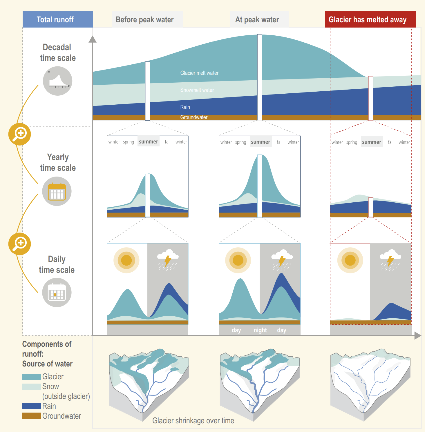
Among other things, climate impacts translate into long-term changes in runoff formation fractions and the distribution of runoff formation within the hydrological year. Figure Figure 6.1 shows a simplified illustration of the changes in runoff regime as glaciers shrink (for the example of a heavily glaciated basin) (Hock et al. 2019). The considerable reduction in river discharge as glaciers disappear from the catchment is noteworthy, especially in the late summer period, which coincides with a period of high irrigation demand in Central Asia. Further, discharge variability is expected to increase; with little to no discharge in late summer when glacier storage is gone and occasional high precipitation runoff due to high intensity rainfall events.
By the end of the century, an average reduction of 50 % to 80 % of glacier mass has to be expected in Central Asia (Marzeion et al. 2020), depending on the socio-economic pathway. Glaciers at low elevations will completely disappear. As the cryosphere acts as a natural seasonal to multi-year water reservoir, the loss of this storage capacity has a large impact on downstream food and energy production and the environment, with associated economic loss (Rasul and Molden 2019).
As a demonstration site, we use the catchment of the gauging station on the Atbashy River, a tributary to the Naryn River in Central Asia. If you’d like to reproduce the examples presented in this Chapter, you can download the zipped data in the example data set available here. You can extract the downloaded data into a location of your choice and adapt the reference path below. The rest of the code will run as it is, provided you have the required r packages installed. The size of the data package is 14.1 GB.
Please note that new (highly relevant and public) glacier data are released ever more frequently. The summary provided here refers to the latest data sets at the time of writing in February 2022.
6.2 Snow Cover and Snow Water Equivalent
We start with the upper-most cryosphere layer: the snow cover. A large amount of data sets are available and the following section presents a suitable product for the calibration of the snow module in the HBV model objects.
6.2.1 High Mountain Asia Snow Reanalysis (HMASR) Product
Yufei Liu, Fang, and Margulis (2021) provide a daily reanalysis product for snow-covered area and snow water equivalent (SWE) in High Mountain Asia between October 1, 1999 and September 30, 2017. The spatial resolution is 16 arc-seconds (approximately 400 m) and the spatial coverage is N: 45, S: 27, E: 105, W: 60 so the northern-most headwater basins of the Illi River catchment are unfortunately not covered. Other SWE products have a coarser spatial resolution (e.g. the Daily Snow Depth Analysis Data by the Canadian Meteorological Center, which is available at 24 km grid resolution). They are thus less suited for calibration of hydrological models of small to medium sized headwater basins.
The HMASR data is available via NSIDC (Y. Liu, Fang, and Margulis 2021). Their SWE can directly be compared to the SWE computed in hydrological models like HBV. More on this in the model calibration section.From the downloaded data, only the SWE and the validity mask (showing the pixels where the snow water equivalent product is valid) is required. Please note that the warning is due to the .nc file format and need not concern you. The SWE data is read correctly from the .nc files.
dem <- raster(paste0(data_path, "GIS/16076_DEM.tif"))
basin <- st_read(paste0(data_path, "GIS/16076_Basin_outline.shp"), quiet = TRUE)

# Load one example file and display SWE for a random date in the cold season.
filespath <- paste0(data_path, "SNOW/")
year <- 1999

# Load non-seasonal snow mask
filepart <- "_MASK.nc"
index = sprintf("%02d", (year - 1999))

# The Atbashy basin is covered by two raster stacks
mask_w <- raster::brick(paste0(filespath,
                               "HMA_SR_D_v01_N41_0E76_0_agg_16_WY",
                               year, "_", index, filepart),
                     varname = "Non_seasonal_snow_mask")
raster::crs(mask_w) = raster::crs("+proj=longlat +datum=WGS84 +no_defs")
mask_e <- raster::brick(paste0(filespath,
                               "HMA_SR_D_v01_N41_0E77_0_agg_16_WY",
                               year, "_", index, filepart),
                     varname = "Non_seasonal_snow_mask")
raster::crs(mask_e) = raster::crs("+proj=longlat +datum=WGS84 +no_defs")

# The rasters need to be rotated
template <- raster::projectRaster(from = mask_e, to= mask_w, alignOnly = TRUE)

# template is an empty raster that has the projected extent of r2 but is
# aligned with r1 (i.e. same resolution, origin, and crs of r1)
mask_e_aligned <- raster::projectRaster(from = mask_e, to = template)
mask_w <- flip(t(mask_w), direction = 'x')
mask_e_aligned <- flip(t(mask_e_aligned), direction = 'x')
mask <- merge(mask_w, mask_e_aligned, tolerance = 0.1)
mask = raster::projectRaster(from = mask,
                             crs = crs("+proj=utm +zone=42 +datum=WGS84 +units=m +no_defs"))

# Load snow data
varname = "SWE_Post"
filepart <- "_SWE_SCA_POST.nc"
sca_w <- raster::brick(paste0(filespath,
                              "HMA_SR_D_v01_N41_0E76_0_agg_16_WY",
                              year, "_", index, filepart),
                       varname = varname, level = 1)
[1] "vobjtovarid4: **** WARNING **** I was asked to get a varid for dimension named Day BUT this dimension HAS NO DIMVAR! Code will probably fail at this point"raster::crs(sca_w) = raster::crs("+proj=longlat +datum=WGS84 +no_defs")
sca_e <- raster::brick(paste0(filespath,
"HMA_SR_D_v01_N41_0E77_0_agg_16_WY",
year, "_", index, filepart),
varname = varname, level = 1)[1] "vobjtovarid4: **** WARNING **** I was asked to get a varid for dimension named Day BUT this dimension HAS NO DIMVAR! Code will probably fail at this point"raster::crs(sca_e) = raster::crs("+proj=longlat +datum=WGS84 +no_defs")
template <- raster::projectRaster(from = sca_e, to = sca_w, alignOnly = TRUE)
# template is an empty raster that has the projected extent of r2 but is
# aligned with r1 (i.e. same resolution, origin, and crs of r1)
sca_e_aligned<- raster::projectRaster(from = sca_e, to = template)
sca_w <- flip(t(sca_w), direction = 'x')
sca_e_aligned <- flip(t(sca_e_aligned), direction = 'x')
sca <- raster::merge(sca_w, sca_e_aligned, tolerance = 0.1)
sca <- projectRaster(from = sca,
crs = crs("+proj=utm +zone=42 +datum=WGS84 +units=m +no_defs"))
sca_masked <- mask(sca, mask, maskvalue = 1)
sca_masked <- mask(sca_masked, basin)
# Visualize snow water equivalent
tmap_mode("view")
tm_shape(max(sca_masked, na.rm = TRUE)) +
tm_raster(n = 6,
palette = "Blues",
alpha = 0.8,
legend.show = TRUE,
title = "SWE (m)") +
tm_shape(basin) +
tm_borders(col = "black", lwd = 0.6)6.2.2 Operational SLF Model Data on Snow Height and Snow Water Equivalent
For operational hydrological modelling, different possibilities exist to obtain near-real time snow cover, height and information on the snow water equivalent (SWE). One such option is to use data from the operational SLF Model.
- February 2024: More information coming soon!
6.3 Glacier Outlines
The Randolph Glacier Inventory (RGI) v6.0 (RGI Consortium 2017) makes a consistent global glacier data base publicly available1. It includes geolocated glacier geometry and some additional parameters like elevation, length, slope and aspect. For water resources modeling in Central Asia, RGI regions 13 (Central Asia) and 14 (South Asia West) are relevant. The glacier geometries for all RGI regions are available from the GLIMS RGI v6.0 website. For this demo, the data for the Atbashy River basin is available from the data download link given above.
# Loading the data
rgi <- st_read(paste0(data_path, "GIS/16076_Glaciers_per_subbasin.shp"),
               quiet = TRUE) |>
  st_transform(crs = crs(dem))

# Generation of figure
tmap_mode("view")
tm_shape(dem, name = "DEM") +
  tm_raster(n = 6,
            palette = terrain.colors(6),
            alpha = 0.8,
            legend.show = TRUE,
            title = "Elevation (masl)") +
  tm_shape(rgi, name = "RGI v6.0") +
tm_polygons(col = "lightgray", lwd = 0.2)6.4 Glacier Thickness
Farinotti et al. (2019) make distributed glacier thickness maps available for each glacier in the RGI v6.0 data set. As the data set is large, we have downloaded the required maps of glacier thickness for you and made them available in the download link above. We will refer to this data set as the glacier thickness data set or the Farinotti data set.
Please note that Farinotti et al. (2019) provide ice thickness. This can be converted to water equivalents by assuming a ice density of 900 kg/m3, e.g. 100 m glacier thickness translates to a water column of about 90 m.
The original glacier thickness data set is available from the data collection of Farinotti et al. (2019) which is available from the data section of their online article.
The following code chunks demonstrates how to extract glacier thickness data from the Farinotti data set.
6.4.1 How to Extract Glacier Thickness
# Get a list of all files in the glacier thickness data set. The files are named
# after the glacier ID in the RGI v6.0 data set (variable RGIId).
glacier_thickness_dir <- paste0(data_path, "GLACIERS/Farinotti/")
filelist <- list.files(path = glacier_thickness_dir, pattern = ".tif$",
                       full.names = TRUE)

# Filter the glacier thickness file list for the glacier ids in the catchment of
# interest.
filelist <- filelist[sapply(rgi$RGIId, grep, filelist)]

# Get the maximum glacier thickness for each of the glaciers in filelist.
# Note: this works only for small catchments as the origin of the rasters to be
# mosaiced needs to be consistent. For a larger data set you will need to implement
# a loop over all glaciers to extract the thickness per glacier or per elevation
# band. This operation can take a while.
glacier_thickness <- Reduce(function(x, y) raster::mosaic(x, y, fun = max),
                            lapply(filelist, raster::raster))

# For plotting, clip the glacier thickness raster of the basin to the basin boundary
glacier_thickness <- mask(glacier_thickness |>
projectRaster(crs = crs(dem)), basin)tmap_mode("view")
tm_shape(dem, name = "DEM") +
tm_raster(n = 6,
palette = terrain.colors(6),
alpha = 0.8,
legend.show = TRUE,
title = "Elevation (masl)") +
tm_shape(glacier_thickness, name = "Farinotti") +
tm_raster(n = 6,
palette = "Blues",
legend.show = TRUE,
title = "Glacier thickness\n(m)") +
tm_shape(rgi, name = "RGI v6.0") +
tm_borders(col = "gray", lwd = 0.4) +
tm_shape(basin, name = "Basin outline") +
tm_borders(col = "black", lwd = 0.6)A more recent glacier thickness data set by Millan et al. (2022) estimates much larger ice reservoirs in the Himalayan region but similar goodness of fit for the glaciers in the Central Asian region as the Farinotti data set. The Millan et al. (2022) data set is not included in the present workflow yet but should be considered as an alternative for the Farinotti data set.
The glacier thickness data set by Farinotti et al. (2019) can for example be combined with the RGI v6.0 data set for the Central Asia region to validate the well-known glacier area-volume relationship by Erasov (1968) (see section Area-Volume scaling).
6.5 Glacier Thinning Rates
Hugonnet et al. (2021) provide annual estimates of glacier thinning rates for each glacier in the RGI v6.0 data set. The authors advise to not to rely on the annual data but rather on an average over at least 5 years to get reliable thinning rates for individual glaciers. We compare trends in glacier thinning rates to trends in glacier thickness during model calibration. We will refer to this data set as the thinning rates data set or the Hugonnet data set. A copy of the Hugonnet thinning rates is included in the download link above.
The original per-glacier time series of thinning rates can be downloaded from the data repository as described in the github site linked under the code availability section of the online paper of Hugonnet et al. (2021).
hugonnet <- read_csv(paste0(data_path, "/GLACIERS/Hugonnet/dh_13_rgi60_pergla_rates.csv"))
# Explanation of variables:
# - dhdt is the elevation change rate in meters per year,
# - dvoldt is the volume change rate in meters cube per year,
# - dmdt is the mass change rate in gigatons per year,
# - dmdtda is the specific-mass change rate in meters water-equivalent per year.

# Filter the basin glaciers from the Hugonnet data set.
hugonnet <- hugonnet |>
  dplyr::filter(rgiid %in% rgi$RGIId) |>
  tidyr::separate(period, c("start", "end"), sep = "_") |>
  mutate(start = as_date(start, format = "%Y-%m-%d"),
         end = as_date(end, format = "%Y-%m-%d"),
         period = round(as.numeric(end - start, units = "days")/366))

# Join the Hugonnet data set to the RGI data set to be able to plot the thinning
# rates on the glacier geometry.
glaciers_hugonnet <- rgi |>
  left_join(hugonnet |> dplyr::select(rgiid, area, start, end, dhdt, err_dhdt,
                                      dvoldt, err_dvoldt, dmdt, err_dmdt,
                                      dmdtda, err_dmdtda, period),
            by = c("RGIId" = "rgiid"))

# Visualization of data
tmap_mode("view")
tm_shape(dem, name = "DEM") +
  tm_raster(n = 6,
            palette = terrain.colors(6),
            alpha = 0.8,
            legend.show = TRUE,
            title = "Elevation (masl)") +
  tm_shape(glaciers_hugonnet |> dplyr::filter(period == 20), name = "Hugonnet") +
  tm_fill(col = "dmdtda",
          n = 6,
          palette = "RdBu",
          midpoint = 0,
          legend.show = TRUE,
          title = "Glacier thinning\n(m weq/a)") +
  tm_shape(rgi, name = "RGI v6.0") +
  tm_borders(col = "light blue", lwd = 0.4) +
  tm_shape(basin, name = "Basin outline") +
tm_borders(col = "black", lwd = 0.6)6.6 Glacier Discharge
Miles et al. (2021) ran specific mass balance calculations over many glaciers larger than 2 km2 in High Mountain Asia (HMA). They provide the average glacier discharge between 2000 and 2016. We will refer to this data set as the glacier discharge data set or the Miles data set. A copy of the glacier discharge data is available from the data download link provided above. The glacier ablation data can be used as a third party data set to validate glacier discharge rates simulated using the GSM model implemented in RS MINERVE.
The original data is available from the data repository linked in the online version of the paper.
glaciers_miles <- read_csv(paste0(data_path, "GLACIERS/Miles/Miles2021_Glaciers_summarytable_20210721.csv")) |>
  dplyr::filter(VALID == 1,
                RGIID %in% glaciers_hugonnet$RGIId)

glaciers_miles <- rgi |>
  left_join(glaciers_miles |>
              dplyr::select(-c(VALID, CenLat, CenLon)),
            by = c("RGIId" = "RGIID"))

# Data visualization
tmap_mode("view")
tm_shape(dem, name = "DEM") +
  tm_raster(n = 6,
            palette = terrain.colors(6),
            alpha = 0.8,
            legend.show = TRUE,
            title = "Elevation (masl)") +
  tm_shape(glaciers_miles, name = "Miles") +
  tm_fill(col = "totAbl",
          n = 6,
          palette = "RdBu",
          midpoint = 0,
          legend.show = TRUE,
          title = "Glacier ablation\n(m3/a)") +
  tm_shape(rgi, name = "RGI v6.0") +
  tm_borders(col = "gray", lwd = 0.4) +
  tm_shape(basin, name = "Glacier outline") +
tm_borders(col = "black", lwd = 0.6)6.7 Glacier Discharge Projections
Projected glacier and off-glacier discharge for the 21th century are provided by Rounce, Hock, and Shean (2020a) through NSIDC. Monthly per-glacier discharge rates for RGI v6.0 region 13 have been produced using the Python Glacier Evolution Model (PyGEM) (Rounce, Hock, and Shean 2020b). PyGEM glacier discharge projections are done using the CMIP 5 climate model ensemble and emission scenarios. These are thus not 1-to-1 compatible with the CMIP6 models and SSP used as climate forcing in this book. Riahi et al. (2017) compare radiative forcing (an important driver for glacier melt) for CMIP5 and CMIP6 scenarios and show that the lower emission CMIP5 scenarios (RCP2 2.4 and RCP 4.5) underestimate radiative forcing as compared to the CMIP6 SSP counterparts (SSP 1 and SSP 2.). This means that also glacier melt simulated using the CMIP5 model ensembles may underestimate actual glacier melt for the lower emission scenarios. RCP 8.5 seems to be, however, fairly compatible with SSP 5. There is no counterpart for SSP 3 in the CMIP5 scenarios.
In 2023, glacier discharge projections using CMIP6 models and scenarios were released (Rounce et al. 2023). These can directly be used in climate impact modeling assessments. We use these PyGEM glacier discharge projections for estimating future glacier melt in the entire Central Asian region.
6.8 A Note on the Uncertainties of the Glacier Data Sets
The geometries of the RGI v6.0 data set are generally very good. If you simulate glacier discharge in a small catchment with few glaciers it is advisable to visually check the glacier geometries and make sure, all relevant glaciers in the basin are included in the RGI data set. You may have to manually add missing glaciers or correct the geometry.
For some regions in Central Asia, OpenStreetMap is an excellent reference for glacier locations and names in Central Asia. You can import the map layer in QGIS or also download individual GIS layers.
The glacier thickness data set is validated only at few locations as measurements of glacier thickness are typically not available. Farinotti et al. (2019) list an uncertainty range for the volume estimate in regions RGI 13 and 14 of 26 % each.
Hugonnet et al. (2021) & Miles et al. (2021) provide the uncertainties of their estimates for per-glacier glacier thinning & discharge rates in the data set itself. They typically lie around \(\pm\) 150%.
6.9 Permafrost Extent
While glaciers are intensively researched, also in Central Asia, little is known about the extent of permafrost in High Mountain Asia and how climate change will impact permafrost regions (Barandun et al. 2020). A high-resolution (1 km grid resolution, average between 2000 and 2016) estimate of permafrost extent is available from the ESA GlobPermafrost program (Obu et al. 2019). Data can be downloaded from the Arctic Permafrost Geospatial Center (APGC). Figure Figure 6.7 shows the permafrost probability extent, i.e. the estimated fraction of grid cell covered by permafrost. Glaciated areas are excluded.
The permafrost probability extent can for example be used to inform model zonation.
# Load the data and cut to the Atbashy basin
permafrost <- raster(paste0(data_path, "PERMAFROST/Permafrost_extent.tif"))

tmap_mode("view")
tm_shape(permafrost, name = "Permafrost") +
  tm_raster(n = 6,
            palette = "Blues",
            legend.show = TRUE,
            title = "Perfafrost prob.\nextent") +
  tm_shape(rgi, name = "RGI v6.0") +
  tm_borders(col = "gray", lwd = 0.4) +
  tm_shape(basin, name = "Basin outline") +
tm_borders(col = "black", lwd = 0.6)7 References
Armstrong, Richard L., Karl Rittger, Mary J. Brodzik, Adina Racoviteanu, Andrew P. Barrett, Siri-Jodha Singh Khalsa, Bruce Raup, et al. 2019. “Runoff from Glacier Ice and Seasonal Snow in High Asia: Separating Melt Water Sources in River Flow.” Regional Environmental Change 19 (5): 1249–61. https://doi.org/10.1007/s10113-018-1429-0.
Barandun, Martina, Joel Fiddes, Martin Scherler, Tamara Mathys, Tomas Saks, Dimitry Petrakov, and Martin Hoelzle. 2020. “The State and Future of the Cryosphere in Central Asia.” Water Security 11. https://doi.org/10.1016/j.wasec.2020.100072.
Erasov, N. V. 1968. “Method for Determining of Volume of Mountain Glaciers.” MGI, no. 14: 307–8.
Farinotti, Daniel, Matthias Huss, Johannes J. Fürst, Johannes Landmann, Horst Machguth, Fabien Maussion, and Ankur Pandit. 2019. “A Consensus Estimate for the Ice Thickness Distribution of All Glaciers on Earth.” Nature Geoscience 12 (3): 168–73. https://doi.org/10.1038/s41561-019-0300-3.
Gruber, Stephan, Renate Fleiner, Emilie Guegan, Prajjwal Panday, Marc-Olivier Schmid, Dorothea Stumm, Philippus Wester, Yinsheng Zhang, and Lin Zhao. 2017. “Review Article: Inferring Permafrost and Permafrost Thaw in the Mountains of the Hindu Kush Himalaya Region.” The Cryosphere 11 (1): 81–99. https://doi.org/10.5194/tc-11-81-2017.
Hock, R., G. Rasul, C. Adler, B. Cáceres, S. Gruber, Y. Hirabayashi, M. Jackson, et al. 2019. “High Mountain Areas. In: IPCC Special Report on the Ocean and Cryosphere in a Changing Climate.” Edited by H.-O. Pörtner, D. C. Roberts, V. Masson-Delmotte, P. Zhai, M. Tignor, E. Poloczanska, K. Mintenbeck, et al.
Hugonnet, Romain, Robert McNabb, Etienne Berthier, Brian Menounos, Christopher Nuth, Luc Girod, Daniel Farinotti, et al. 2021. “Accelerated Global Glacier Mass Loss in the Early Twenty-First Century.” Nature 592 (7856): 726–31. https://doi.org/10.1038/s41586-021-03436-z.
Kaser, G., M. Grosshauser, and B. Marzeion. 2010. “Contribution Potential of Glaciers to Water Availability in Different Climate Regimes.” Proceedings of the National Academy of Sciences 107 (47): 20223–27. https://doi.org/10.1073/pnas.1008162107.
Khanal, S., A. F. Lutz, P. D. A. Kraaijenbrink, B. van den Hurk, T. Yao, and W. W. Immerzeel. 2021. “Variable 21st Century Climate Change Response for Rivers in High Mountain Asia at Seasonal to Decadal Time Scales.” Water Resources Research 57 (5). https://doi.org/10.1029/2020WR029266.
Liu, Y., Y. Fang, and S. A. Margulis. 2021. “High Mountain Asia UCLA Daily Snow Reanalysis.” Boulder, Colorado USA: NASA National Snow; Ice Data Center Distributed Active Archive Center. doi: https://doi.org/10.5067/HNAUGJQXSCVU.
Liu, Yufei, Yiwen Fang, and Steven A. Margulis. 2021. “Spatiotemporal Distribution of Seasonal Snow Water Equivalent in High-Mountain Asia from an 18-Year Landsat-MODIS Era Snow Reanalysis Dataset.” The Cryosphere 15: 5261–80. https://doi.org/10.5194/tc-2021-139.
Marzeion, Ben, Regine Hock, Brian Anderson, Andrew Bliss, Nicolas Champollion, Koji Fujita, Matthias Huss, et al. 2020. “Partitioning the Uncertainty of Ensemble Projections of Global Glacier Mass Change.” Earth’s Future 8 (7). https://doi.org/10.1029/2019EF001470.
Miles, Evan, Michael McCarthy, Amaury Dehecq, Marin Kneib, Stefan Fugger, and Francesca Pellicciotti. 2021. “Health and Sustainability of Glaciers in High Mountain Asia.” Nature Communications 12 (2868): 10. https://doi.org/https://doi.org/10.1038/s41467-021-23073-4.
Millan, Romain, Jérémie Mouginot, Antoine Rabatel, and Mathieu Morlighem. 2022. “Ice Velocity and Thickness of the World’s Glaciers.” Nature Geoscience 15 (2): 124–29. https://doi.org/10.1038/s41561-021-00885-z.
Obu, Jaroslav, Sebastian Westermann, Annett Bartsch, Nikolai Berdnikov, Hanne H. Christiansen, Avirmed Dashtseren, Reynald Delaloye, et al. 2019. “Northern Hemisphere Permafrost Map Based on TTOP Modelling for 2000 at 1 Km2 Scale.” Earth-Science Reviews 193 (June): 299–316. https://doi.org/10.1016/j.earscirev.2019.04.023.
Rasul, Golam, and David Molden. 2019. “The Global Social and Economic Consequences of Mountain Cryospheric Change.” Frontiers in Environmental Science 7 (June): 91. https://doi.org/10.3389/fenvs.2019.00091.
RGI Consortium. 2017. “Randolph Glacier Inventory – a Dataset of Global Glacier Outlines: Version 6.0: Technical Report.” Global Land Ice Measurements from Space, Colorado, USA. Digital Media. https://doi.org/https://doi.org/10.7265/N5-RGI-60.
Rounce, David R., Regine Hock, Fabien Maussion, Romain Hugonnet, William Kochtitzky, Matthias Huss, Etienne Berthier, et al. 2023. “Global Glacier Change in the 21st Century: Every Increase in Temperature Matters.” Science 379 (6627): 7883. https://doi.org/10.1126/science.abo1324.
Rounce, David R., Regine Hock, and David E. Shean. 2020a. “High Mountain Asia PyGEM Glacier Projections with RCP Scenarios.” Data Set. NASA National Snow and Ice Data Center Distributed Active Archive Center. https://doi.org/10.5067/190Y84IGLIQH.
———. 2020b. “Glacier Mass Change in High Mountain Asia Through 2100 Using the Open-Source Python Glacier Evolution Model (PyGEM).” Frontiers in Earth Science 7 (January): 331. https://doi.org/10.3389/feart.2019.00331.