# Core Libraries
install.packages('tidyverse') # Meta - dplyr, ggplot2, purrr, tidyr, stringr, forcats
install.packages('lubridate') # date and time
install.packages('timetk') # Time series data wrangling, visualization and preprocessing
install.packages('modeltime') # latest and greatest time series modeling package for R
install.packages('tidymodels') # The tidymodels framework is a collection of packages for modeling and machine learning using tidyverse principles.
# Sample data from Central Asia river basins and helper functions
library('devtools')
devtools::install_github("hydrosolutions/riversCentralAsia")10 Modeling Using Predictive Inference
10.1 Prerequisites
Time series-based hydrological models use past discharge observations and auxilliary variables such as snow cover in the catchment and/or precipitation to predict the future from learned past patterns. Currently, no ready-made hydrological modeling packages can be used for this purpose. Such types of models rather draw on available time series-based modeling algorithms that are implemented and available in dedicated packages for programming environments like R.
We will work with R and RStudio and the following packages that need to be installed to replicate and run the models shown here. Note that such a package installation step only has to be performed once.
The packages can then be loaded and made available in your R session.
When other additional packages are needed, they will be loaded in the corresponding Sections below.
Please also remember the following rules when working with R dataframes in the tidyverse:
- Every column is variable.
- Every row is an observation.
- Every cell is a single value.
A final note. In all of the following, we mostly use the powerful data manipulation and visualization techniques for time series data as provided by the timetk package. This package greatly facilitates any work with time series data as it, among other things, nicely integrates with the R ‘tidyverse’.
10.2 Forecasting Using Predictive Inference
In this Section, we are concerned with predictive inference using observed data to predict future data that is not known yet but that is important to forecast with high confidence and low uncertainty. In other words, it is assumed that we can encapsulate historic patterns in a model for learning about the future with such model.
In hydrology, we are dealing with time series, i.e. ordered observations in time. A generic model structure thus can be specified in the following way
\[ y(t+\Delta t) = f(y(t),x(t)) + \epsilon(t) \]
where \(y(t+\Delta t)\) is called the forecast target (discharge at a particular gauge in our case) and is the variable that we want to forecast in the future, i.e. \(\Delta t\) time away from now. \(y(t)\) denotes past known observations of discharge up and including time \(t\). Similarly, \(x(t)\) denotes other variables of interest, called external regressors, that might be relevant to obtain good quality forecasts such as meteorological data from local stations, including precipitation and temperature. Finally, \(f()\) denotes the type of model that is being used for forecasting and \(\epsilon\) are the time-dependent error terms. If, for example, one would use a linear modeling approach without external regressors, such type of model could simply be written as
\[ y(t+\Delta t) = \beta_{0} + \beta_{1} \cdot y(t) + \epsilon(t) \]
In the model specification above, the aim is to predict the future with a lead time of \(\Delta t\), i.e., for example one month ahead. The lead-time model can be written in equivalent form using lags in the following way
\[ y(t) = f(y(t-lag),x(t-lag)) + \epsilon(t) \]
where \(lag = \Delta t\). This just means that we use all the available observations until and including \(t-lag\) for predicting the target at the time \(t\). We will use these specifications throughout the Chapter when working with and developing new forecasting models.
10.3 Forecasting Discharge in Central Asian
10.3.1 Hydrometeorological Organizations
The key agencies that are charged in predicting river discharge regularly are the Central Asia National Meteorological and Hydrological Services (NMHS). For the prediction of mean discharge over a specific target future period, they use different types of statistical models.
The particular type of model they use depends on the available hydrological and meteorological data for a particular river whose mean discharge is to be forecasted and on the type of the forecast. Types of forecasts include
- daily forecasts, i.e. \(\Delta t = 1 \text{ day}\),
- pentadal forecasts, i.e. \(\Delta t = 5 \text{ days}\),
- decadal forecasts, i.e. \(\Delta t = 10 \text{ days}\),
- monthly forecasts, i.e. \(\Delta t = 1 \text{ month}\), and
- seasonal forecasts, i.e. \(\Delta t = 6 \text{ months}\).
To this date, these types of forecasts are performed at regular intervals by the operational hydrologists. Normally, this requires a lot of manual work. Recently, selected NMHS use automated software to automatize this type of work. The Chapter on Real-World Hydrological Modeling Applications discusses such a software application, called iEasyHydro, in greater detail.
In Uzbekistan, for example, the following list of forecast objects exists in the NMHS.
| River | Gauge (Target Object) | Gauge Code | Country | Types of Forecasts |
|---|---|---|---|---|
| Chirchik | Inflow to Charvak Res. | 16924 | UZB | dl, m, s |
| Chirchik | Inflow to Charvak Res. + Ugam River | 16924 + 16300 | UZB | m, s |
| Akhangaran | Irtash | 16230 | UZB | m, s |
| Chadak | Dzhulaysay | 16202 | UZB | m, s |
| Gavasay | Gava | 16193 | UZB | m, s |
| Padsha-Ata | Tostu | 16176 | KGZ | m, s |
| Kara Darya | Inflow to Andizhan water reservoir | 16938 | UZB/KGZ | dl, m, s |
| Isfayramsoy | Uch-Kurgan | 16169 | KGZ | m, s |
| Sokh | Sarykanda | 16198 | UZB | dl (May - Sep.), m, s |
| Sanzar | Kyrk | 16223 | UZB | m, s |
| Naryn | Inflow to Toktogul water reservoir | 16936 | KGZ | m, s |
| Vaksh | Inflow to Nurek water reservoir | 17084 (Vakh river - Darband gauge) | TJK | m, s |
| Kafirnigan | Tartki | 17137 | TJK | m, s |
| Tupalang | Inflow to Tupalang water reservoir | 17194 | UZB | m, s |
| Sangardak | Keng-Guzar | 17211 | UZB | m, s |
| Akdarya | Inflow to Gissarak water reservoir | 17464 (Akfariya river - Hissarak gauge) | UZB | m, s |
| Yakkabagdarya | Tatar | 17260 | UZB | m, s |
| Uryadariya + Kichik Uryadariya | Inflow to Pachkamar water reservoir | 17279 (Uryadariya river - Bazartepe gauge) + 17275 (Kichik Uryadariya - Gumbulak gauge) | UZB | m, s |
| Zeravshan | Inflow to Rovatkhodzha hydro work | 17461 | UZB | m, s |
It should be noted that all of the NMHS have lists with different forecast targets for different rivers. As can be seen from the above list, Uzbekistan does not issue pentade and decadal forecasts, i.e. types of forecasts, which are regularly issued by the KGZ, for example.
Finally, seasonal forecasts in the Uzbek NMHS are issued twice before the irrigation season with 3. - 5. March being the first data range for issuing, and 3. - 5. April being the second one. Converse to this, monthly forecasts are issues between the 25. - 27. day each month. Finally, decadal and pentade forecasts are issued each morning at the day of the end of the corresponding pentade or decade.
It is important to emphasize again that there is currently no standardized way in the region to produce these forecasts. While in some instances, a particular approach and method works very well, it fails to produce acceptable forecasts in other basins. However, as we shall see, certain techniques work very well for particular forecast horizons which then explains why such type of technique has become widely used in the region.
10.3.2 Forecasting for What and Whom?
Why is all this work is required? What is the purpose of predicting mean discharge into the future at regular intervals? Important recipients of the forecast products include the Water Authorities which are in charge of delivering adequate amounts of water for irrigation at the right time and location.
It all starts with pre-season irrigation planning. The main irrigation season in most of Central Asia is from April 1. through the end of September. Previous to the start of the irrigation season, irrigation plans are drafted based on computed irrigation water demand of all the water users that are connected to a particular irrigation system. These irrigation system are defined in terms of canal topology where demand gets aggregated from the bottom up to the Rayvodkhozes and the Oblvodkhozes. The later then starts with the pre-season irrigation planning given the water irrigation system-level demand. These plans specify decadal water discharge for each irrigation system and the corresponding canals.
Demand is one thing, but expected supply from the Central Asian rivers another. In order to be able to match the irrigation water demand, the water authorities do what is needed and receive from the Hydromets first the seasonal discharge forecasts. Given this forecast of irrigation-season water availability, the water authorities then adjust their plans given the particular expected circumstances. If, for example, an exceptionally dry year is expected, they activate limit plans and reduce planned water distributions according to forecasted quantities. If a wet year is expected, they do not perform these adjustments and maybe even release water from reservoirs previous to the irrigation season to ensure enough storage capacity in the reservoirs.
With the beginning of the irrigation season, another seasonal forecast is carried out by the Hydromets and communicated to the Central Asian water authorities. Given the updated forecast, planning is revised and adjusted accordingly. Then, finally, throughout the irrigation season pentadal, decadal and monthly forecasts are produced constantly to carefully balance water demand with supplies while the season is under way.
Needless to say that other important customers for hydrometeorological forecasts exist, including for example airports, road departments that need to ensure road safety, agricultural clusters that are interested in frost and hail warnings, local authorities that need to be alerted in the case of extreme local weather conditions, etc.
10.4 Data and Preparation
10.4.1 Available Data
The riversCentralAsia Package provides available data of the gauging and meteorological stations in the Chirchik River Basin.
Before starting any type of modeling, it is important to get a good understanding of the data that we are dealing with and whether there exist problems with the raw data that need to be addressed prior to modeling. Problems usually include data gaps and outliers as data record that one obtains are usually ever complete nor clean of errors.
The steps performed here are thus required steps for any type of successful modeling and should be performed with great care. We concentrate our efforts here on discharge records and data from meteorological stations in the Chirchik River Basin. The techniques shown here for decadal (10-days) data naturally extend to monthly data and other basins.
10.4.2 Gap Filling Discharge Data
In the following, we will work with decadal discharge data from the two main tributaries, i.e. the Chatkal and (Gauge 16279) Pskem rivers (Gauge 16290) and the data of the inflow to the Charvak reservoir (Gauge 16924). The goal is to analyze the data and prepare for modeling. First, let us load the relevant discharge data.
data <- ChirchikRiverBasin # load data
q_dec_tbl <- data |> filter(code == '16279' | code == '16290' | code == '16924') # Note for the new name of the object, we choose to add periodicity (_dec_) and data type (_tbl for tibble/dataframe) to the data name. This just helps to stay organized and is good practice in R programming.
q_dec_tbl# A tibble: 9,072 × 14
date data norm units type code station river basin resolution
<date> <dbl> <dbl> <chr> <fct> <chr> <chr> <chr> <chr> <fct>
1 1932-01-10 48.8 38.8 m3s Q 16279 Khudaydod Chatkal Chirch… dec
2 1932-01-20 48.4 37.5 m3s Q 16279 Khudaydod Chatkal Chirch… dec
3 1932-01-31 42.4 36.6 m3s Q 16279 Khudaydod Chatkal Chirch… dec
4 1932-02-10 43.7 36.4 m3s Q 16279 Khudaydod Chatkal Chirch… dec
5 1932-02-20 44.2 36.3 m3s Q 16279 Khudaydod Chatkal Chirch… dec
6 1932-02-29 47.7 36.9 m3s Q 16279 Khudaydod Chatkal Chirch… dec
7 1932-03-10 54.1 39.4 m3s Q 16279 Khudaydod Chatkal Chirch… dec
8 1932-03-20 63.2 47.6 m3s Q 16279 Khudaydod Chatkal Chirch… dec
9 1932-03-31 103 60.5 m3s Q 16279 Khudaydod Chatkal Chirch… dec
10 1932-04-10 103 86.4 m3s Q 16279 Khudaydod Chatkal Chirch… dec
# ℹ 9,062 more rows
# ℹ 4 more variables: lon_UTM42 <dbl>, lat_UTM42 <dbl>, altitude_masl <dbl>,
# basinSize_sqkm <dbl>You can get more information about the available data by typing ?ChirchikRiverBasin.
It is advisable to check at this stage for missing data in time series and to fill gaps where present. As can be seen in Figure 10.1, close inspection of the time series indeed reveals some missing data in the 1940ies.
q_dec_tbl |> plot_time_series(date,data,
.facet_vars = code,
.smooth = FALSE,
.interactive = TRUE,
.x_lab = "Date",
.y_lab = "Discharge [m3/s]",
.title = ""
)Note, Figure 10.1 and the following Figures are interactive, so you can zoom in to regions of interest.
Missing data are also confirmed by the warning that the function timetk::plot_time_series() throws (suppressed here). Statistics of the missing data can be easily obtained. As the Table below shows, we can do this analysis for each discharge station separately.
# print knitr::kable table
q_dec_tbl |> group_by(code) |>
summarize(n.na = sum(is.na(data)), na.perc = n.na/n()*100) |>
knitr::kable(caption = "Number of missing data points and percentage of missing data for each discharge station. n.na: number of missing data points in the time series, na.perc: percentage of missing data.")| code | n.na | na.perc |
|---|---|---|
| 16279 | 15 | 0.4960317 |
| 16290 | 39 | 1.2896825 |
| 16924 | 42 | 1.3888889 |
Summarizing the number of observation with missing data reveals 15 data points for station 16279 (0.5 % of total record length) and 39 for station 16290 (1.3 % of total record length). As there are only very few gaps in the existing time series, we use a simple method to fill these. Wherever there is a gap, we fill in the corresponding decadal norm as stored in the norm column in the object q_dec_tbl. The visualization of the results confirms that our simple gap filling approach is indeed satisfactory as shown in Figure 10.2.
q_dec_filled_tbl <- q_dec_tbl
q_dec_filled_tbl$data[is.na(q_dec_filled_tbl$data)] =
q_dec_filled_tbl$norm[is.na(q_dec_filled_tbl$data)] # Gap filling step
q_dec_filled_tbl |> plot_time_series(date, data,
.facet_vars = code,
.smooth = FALSE,
.interactive = TRUE,
.x_lab = "year",
.y_lab = "m^3/s",
.title = ""
)A note of caution here. This simple gap filling technique reduces variance in the time series. It should only be used when the percentage of missing data is low. As will be discussed in the next Section 10.4.3 below, better techniques have to be utilized when there exist substantial gaps and in the case of less regular data.
Finally, we discard the norm data which we used for gap filling of the missing discharge data and convert the data to wide format (see the Table below) to add to it meteorological data in the next Section.
q_dec_filled_wide_tbl <- q_dec_filled_tbl |> # again we use the name convention of objects as introduced above
mutate(code = paste0('Q',code |> as.character())) |> # Since we convert everything to long form, we want to keep information as compact as possible. Hence, we paste the type identifier (Q for discharge here) in from of the 5 digit station code.
dplyr::select(date,data,code) |> # ... and then ditch all the remainder information
pivot_wider(names_from = "code",values_from = "data") # in order to pivot to the long format, we need to make a small detour via the wide format.
q_dec_filled_long_tbl <- q_dec_filled_wide_tbl |> pivot_longer(-date) # and then pivot back
q_dec_filled_wide_tbl# A tibble: 3,024 × 4
date Q16279 Q16290 Q16924
<date> <dbl> <dbl> <dbl>
1 1932-01-10 48.8 38.3 87.1
2 1932-01-20 48.4 37.7 86.1
3 1932-01-31 42.4 36.2 78.6
4 1932-02-10 43.7 35.6 79.3
5 1932-02-20 44.2 35 79.2
6 1932-02-29 47.7 37.1 84.8
7 1932-03-10 54.1 43.1 97.2
8 1932-03-20 63.2 47 110
9 1932-03-31 103 72.1 175
10 1932-04-10 103 73.2 176
# ℹ 3,014 more rowsAs a result, we now have a complete record of decadal discharge data for the two main tributaries of the Chirchik river and the inflow time series to Charvak Reservoir from the beginning of 1932 until and including 2015, i.e. 84 years. The same type of preparatory analysis will now be carried out for the meteorological data.
10.4.3 Gap Filling of Meteorological Data
Here, we use precipitation and temperature data from Pskem (38462), Chatkal (38471) and Charvak Reservoir (38464) Meteorological Stations (see the Example River Basins Chapter for more information on these stations). We also have data from Oygaing station (Station Code 38339) but the record only starts in 1962 and the time resolution is monthly. Therefore, we do not take this station into account here for the time being.
We start with precipitation and plot the available data.
p_dec_tbl <- data |> filter(type=="P" & code!="38339")
p_dec_tbl |> plot_time_series(date,data,
.facet_vars = code,
.interactive = TRUE,
.smooth = FALSE,
.title = "",
.y_lab = "mm/decade",
.x_lab = "year"
)The precipitation data from these 3 stations shows some significant data gaps. The Chatkal Meteorological Station that is located in Kyrgyzstan apparently did not work in the post-transition years and continuous measurements were only resumed there in 1998.
Let us see what happens if we were to use the same simple gap filling technique that we introduced above for discharge.
p_dec_filled_tbl <- p_dec_tbl
p_dec_filled_tbl$data[is.na(p_dec_filled_tbl$data)] = p_dec_filled_tbl$norm[is.na(p_dec_filled_tbl$data)]
p_dec_filled_tbl |> plot_time_series(date,data,
.facet_vars = code,
.interactive = TRUE,
.smooth = FALSE,
.title = "",
.y_lab = "mm/decade",
.x_lab = "year"
)Closely inspect the significant data gap in the 1990ies at Station 38741 (tip: play around and zoom into the time series in the 1990ies in Figure 10.3 and comparing it with the resulting gap-filled timeseries in Figure 10.4. We see that our technique of gap filling with long-term norms is not suitable for this type of data and the significant gap size. The effect of variance reduction is also clearly visible.
Hence, we resort to a more powerful gap filling technique that uses a (regression) model to impute the missing values from existing ones at the neighboring stations, i.e. Stations 38462 and 38464. To do so, we utilize an R package that is tightly integrated in the tidyverse. Please note that if you do not have the required package installed locally, you should install it prior to its use with the following command install.packages('simputation')
library(simputation)
# First, we bring the data into the suitable format.
p_dec_wide_tbl <- p_dec_tbl |>
mutate(code = paste0('P',code |> as.character())) |>
dplyr::select(date,data,code) |>
pivot_wider(names_from = "code",values_from = "data")
# Second, we impute missing values.
p_dec_filled_wide_tbl <- p_dec_wide_tbl |>
impute_rlm(P38471 ~ P38462 + P38464) |> # Imputing precipitation at station 38471 using a robust linear regression model
impute_rlm(P38462 ~ P38471 + P38464) |> # Imputing precipitation at station 38462 using a robust linear regression model
impute_rlm(P38464 ~ P38462 + P38471) # Imputing precipitation at station 38464 using a robust linear regression model
p_dec_filled_long_tbl <- p_dec_filled_wide_tbl |> pivot_longer(c('P38462','P38464','P38471'))
p_dec_filled_long_tbl|> plot_time_series(date,value,
.facet_vars = name,
.interactive = TRUE,
.smooth = FALSE,
.title = '',
.y_lab = "mm/decade",
.x_lab = "year"
)As you can see, we use simple linear regression models to impute missing value in the target time series using observations from the neighboring stations.
Through simple visual inspection, it becomes clear that this type of regression model for gap filling is better suited than the previous approach chosen. Let us check whether we could successfully fill all gaps with this robust linear regression approach.
# Write knitr::kable Table
p_dec_filled_long_tbl |>
group_by(name) |>
summarize(n.na = sum(is.na(value)), n.na.perc = n.na/n()*100) |>
knitr::kable(caption = "Number of missing values and their percentage in the precipitation time series after gap filling.")| name | n.na | n.na.perc |
|---|---|---|
| P38462 | 12 | 0.4016064 |
| P38464 | 12 | 0.4016064 |
| P38471 | 3 | 0.1004016 |
It turns out that we still have very few gaps to deal with. We can see them by simply visualizing the wide tibble. The problem persisted at times when two or more values were missing across the available stations at the same time and where thus the linear regression could not be carried out.
p_dec_filled_wide_tbl |> head(10)# A tibble: 10 × 4
date P38462 P38464 P38471
<date> <dbl> <dbl> <dbl>
1 1933-01-10 NA NA 2
2 1933-01-20 NA NA 10
3 1933-01-31 NA NA 5
4 1933-02-10 NA NA 33
5 1933-02-20 NA NA 8
6 1933-02-28 NA NA 10
7 1933-03-10 NA NA 31
8 1933-03-20 NA NA 50
9 1933-03-31 NA NA 6
10 1933-04-10 23 21.3 13p_dec_filled_wide_tbl |> tail()# A tibble: 6 × 4
date P38462 P38464 P38471
<date> <dbl> <dbl> <dbl>
1 2015-11-10 72 81 19
2 2015-11-20 122 76 43
3 2015-11-30 7 2 3
4 2015-12-10 NA NA NA
5 2015-12-20 NA NA NA
6 2015-12-31 NA NA NAWe can solve the issues related to the missing values at the start of the observation record by using the same technique as above and by only regressing P38462 and P38464 on P38471.
p_dec_filled_wide_tbl <- p_dec_filled_wide_tbl |>
impute_rlm(P38462 ~ P38471) |> # Imputing precipitation at station 38462 using a robust linear regression model
impute_rlm(P38464 ~ P38471) # Imputing precipitation at station 38464 using a robust linear regression model
p_dec_filled_wide_tbl |> head(10)# A tibble: 10 × 4
date P38462 P38464 P38471
<date> <dbl> <dbl> <dbl>
1 1933-01-10 5.60 5.08 2
2 1933-01-20 18.3 16.7 10
3 1933-01-31 10.4 9.46 5
4 1933-02-10 54.9 50.3 33
5 1933-02-20 15.2 13.8 8
6 1933-02-28 18.3 16.7 10
7 1933-03-10 51.8 47.3 31
8 1933-03-20 82.0 75.0 50
9 1933-03-31 12.0 10.9 6
10 1933-04-10 23 21.3 13Converse to this, the complete set of observations is missing for December 2015. We will thus remove these non-observations from our tibble.
# A tibble: 6 × 4
date P38462 P38464 P38471
<date> <dbl> <dbl> <dbl>
1 2015-10-10 5 1 0
2 2015-10-20 89 108 58
3 2015-10-31 34 40 12
4 2015-11-10 72 81 19
5 2015-11-20 122 76 43
6 2015-11-30 7 2 3p_dec_filled_long_tbl <- p_dec_filled_wide_tbl |> pivot_longer(-date)Inspecting the temperature data, we see similar data issues as in the precipitation data set.
t_dec_tbl <- data |> filter(type=="T")
t_dec_tbl |> plot_time_series(date,data,
.facet_vars = code,
.interactive = TRUE,
.smooth = FALSE,
.title = '',
.y_lab = "Mean decadal temperature (°C)",
.x_lab = "Date"
)# First, we bring the data into the suitable format.
t_dec_wide_tbl <- t_dec_tbl |>
mutate(code = paste0('T',code |> as.character())) |>
dplyr::select(date,data,code) |>
pivot_wider(names_from = "code",values_from = "data")
# Second, we impute missing values.
t_dec_filled_wide_tbl <- t_dec_wide_tbl |>
impute_rlm(T38471 ~ T38462) |> # Imputing precipitation at station 38471 using a robust linear regression model
impute_rlm(T38462 ~ T38471) # Imputing precipitation at station 38462 using a robust linear regression model
t_dec_filled_long_tbl <- t_dec_filled_wide_tbl |>
pivot_longer(c('T38462','T38471'))
t_dec_filled_long_tbl|>
plot_time_series(date,value,
.facet_vars = name,
.interactive = TRUE,
.smooth = FALSE,
.title = '',
.y_lab = "Mean decadal temperature (°C)",
.x_lab = "Date"
)There are some irregularities in the temperature time series of Chatkal Meteorological Station in the first decade of the 20th century (tip: zoom in to see these more clearly). Note that these were not introduced by the gap filling technique that we used but are most likely wrong temperature readings. We will return to these in the outlier analysis below in Section 10.4.4.
t_dec_filled_long_tbl |>
group_by(name) |>
summarize(n.na = sum(is.na(value)), n.na.perc = n.na/n()*100) |>
knitr::kable(caption = "Number of missing values and their percentage in the temperature time series after gap filling.")| name | n.na | n.na.perc |
|---|---|---|
| T38462 | 3 | 0.1004016 |
| T38471 | 3 | 0.1004016 |
To see where the missing value are, we find them easily again by looking at the head and tail of the tibble.
t_dec_filled_wide_tbl |> head()# A tibble: 6 × 3
date T38462 T38471
<date> <dbl> <dbl>
1 1933-01-10 -6.9 -16.6
2 1933-01-20 -6.1 -15.5
3 1933-01-31 -6.3 -15.6
4 1933-02-10 -2 -8.6
5 1933-02-20 -3.3 -12.5
6 1933-02-28 -0.1 -8.5t_dec_filled_wide_tbl |> tail()# A tibble: 6 × 3
date T38462 T38471
<date> <dbl> <dbl>
1 2015-11-10 2.4 -2.5
2 2015-11-20 2 -2.2
3 2015-11-30 4.6 -3.7
4 2015-12-10 NA NA
5 2015-12-20 NA NA
6 2015-12-31 NA NA Finally, we remove the non observations again as above with the function na.omit.
t_dec_filled_wide_tbl <- t_dec_filled_wide_tbl |> na.omit()
t_dec_filled_long_tbl <- t_dec_filled_wide_tbl |> pivot_longer(-date)To deal with the missing values at the end of the observational record, we could also have used any other technique. Using the norm values however would have artificially reduced the variance in both cases as explained above. Furthermore and at least in the case of temperature, it is also questionable to what extent a norm calculated over the last 84 years is still representative given global warming. We will look in this important and interesting topic in the next section.
10.4.4 Anomalies and Outliers
We use the function timetk::plot_anomaly_diagnostics to investigate anomalies in the time series. For discharge, we first log-transform the raw data with the following transformation to reduce the variance of the original data.
\[ \hat{q}(t) = log(q(t) + 1) \]
where \(\hat{q}(t)\) denotes the transformed discharge. Prior to the log transformation, 1 is added so as to avoid cases where discharge would be 0 and the logarithmic transform thus undefined. The transformation can easily be done with the log1p() function in R. Backtransformation via the function expm1() simply involves taking the exponent and subtracting 1 from the result.
The exceptionally wet year 19169 shows up as anomalous in the Chatkal River Basin and at the downstream Charvak Reservoir inflow gauge. Figure 10.8 and Figure 10.9 show anomalies diagnostics of the available data.
q_dec_filled_long_tbl |>
plot_anomaly_diagnostics(date,
value |> log1p(),
.facet_vars = name,
.frequency = 36,
.interactive = TRUE,
.title = "",
.x_lab = "Date",
.y_lab = "Log-transformed discharge (log(m³/s))")The investigation of precipitation anomalies shows a succession of regular anomalous wet events over time. It is interesting to see that the winter 1968/69 regularly anomalous at all three stations (Figure @ref(fig:EManomaliesP), zoom in to investigate).
p_dec_filled_long_tbl |>
plot_anomaly_diagnostics(date,
value,
.facet_vars = name,
.interactive = TRUE,
.title = "",
.x_lab = "Date",
.y_lab = "Precipitation (mm)")While intuitively, we would have expected an eceptionally mild winter in 1968/69 due to the precipitation excess, the corresponding anomaly does not show up in the temperature record as shown in Figure 10.10.
t_dec_filled_long_tbl |>
plot_anomaly_diagnostics(date,value,
.facet_vars = name,
.interactive = TRUE,
.title = "",
.x_lab = "Date",
.y_lab = "Temperature (°C)")Apart from the identification of extremal periods since as the 1969 discharge year in the Chatkal river basin, the diagnostics of anomalies also helps to identify likely erroneous data records. In Figure 10.10, for example, when we zoom into the data of the series T38471 in the first decade of the 21st century, problems in relation to positive anomalies during the winter are visible in 4 instances. One explanation would be that in at least some instances, the data are erroneously recorded as positive values when in fact they were negative (see dates ‘2002-01-31’, ‘2005-01-10’ and ‘2007-02-28’, Chatkal Station 38471).
10.4.5 Putting it all Together
Finally, we are now in the position to assemble all data that we will use for empirical modeling. The data is stored in long and wide form and used accordingly where required. For example, in Section @ref{TimeSeriesReg}, we are working with the wide data format to investigate model features in linear regression. Note that we also add a column with a decade identifier. Its use will become apparent in the Section @ref(Chap9FeatureEngineering) below.
# Final concatenation
data_wide_tbl <- right_join(q_dec_filled_wide_tbl,p_dec_filled_wide_tbl,by='date')
data_wide_tbl <- right_join(data_wide_tbl,t_dec_filled_wide_tbl,by='date')
# Add period identifiers (decades in this case)
s <- data_wide_tbl$date |> first()
e <- data_wide_tbl$date |> last()
decs <- decadeMaker(s,e,'end')
decs <- decs |> rename(per=dec)
data_wide_tbl <- data_wide_tbl |> left_join(decs,by='date')
# Creating long form
data_long_tbl <- data_wide_tbl |>
pivot_longer(-date)
# Cross checking completeness of record
data_long_tbl |>
group_by(name) |>
summarize(n.na = sum(is.na(value)), n.na.perc = n.na/n()*100) |>
knitr::kable()| name | n.na | n.na.perc |
|---|---|---|
| P38462 | 0 | 0 |
| P38464 | 0 | 0 |
| P38471 | 0 | 0 |
| Q16279 | 0 | 0 |
| Q16290 | 0 | 0 |
| Q16924 | 0 | 0 |
| T38462 | 0 | 0 |
| T38471 | 0 | 0 |
| per | 0 | 0 |
A consistent data record from 1933 until and including November 2015 is now prepared^Please note that by using left_join above, we have cut off discharge data from the year 1932 since we do not have meteorological data there.^. Let us analyze these data now.
10.5 Data Analysis
In this Section, the goal is to explore and understand the available time series data and their relationships and to take the necessary steps towards feature engineering. Features are predictors that we want to include in our forecasting models that are powerful in the sense that they help to improve the quality of forecasts in a significant manner. Sometimes, the modeler also wants to include synthetic features, i.e. predictors that are not observed but for example derived from observations.
Different techniques are demonstrated that allow us to get familiar with the data that we are using. While we are interested to model discharge of Chatkal and Pskem rivers, it should be emphasized that all the techniques utilized for forecasting easily carry over to other rivers and settings.
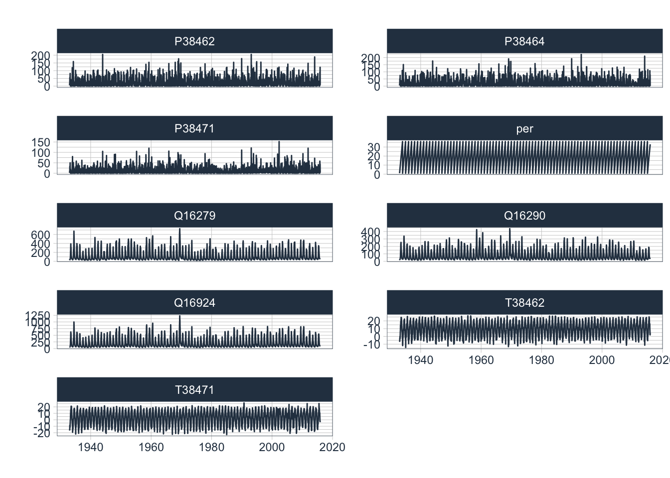
Let us start with a visualisation of the complete data record. Using timetk::plot_time_series and groups, we can plot all data into separate, individual facets as shown in Figure @ref(fig:completeDataRecord).
data_long_tbl |>
group_by(name) |>
plot_time_series(date, value,
.smooth = FALSE,
.interactive = FALSE,
.facet_ncol = 2,
.title = ""
)
10.5.1 Data Transformation
It is interesting to observe that discharge values range over 2 - 3 orders of magnitude between minimum and maximum flow regimes. As can be seen in Figure 10.12, discharge and precipitation data are heavily skewed. When this is the case, it is generally advisable to consider data transformations as they help to improve predictive modeling accuracy of regression models.
data_long_tbl |>
group_by(name) |>
ggplot(aes(x=value,colour = name)) +
geom_histogram(bins=50) +
facet_wrap(~name, scales = "free") +
theme(legend.position = "none")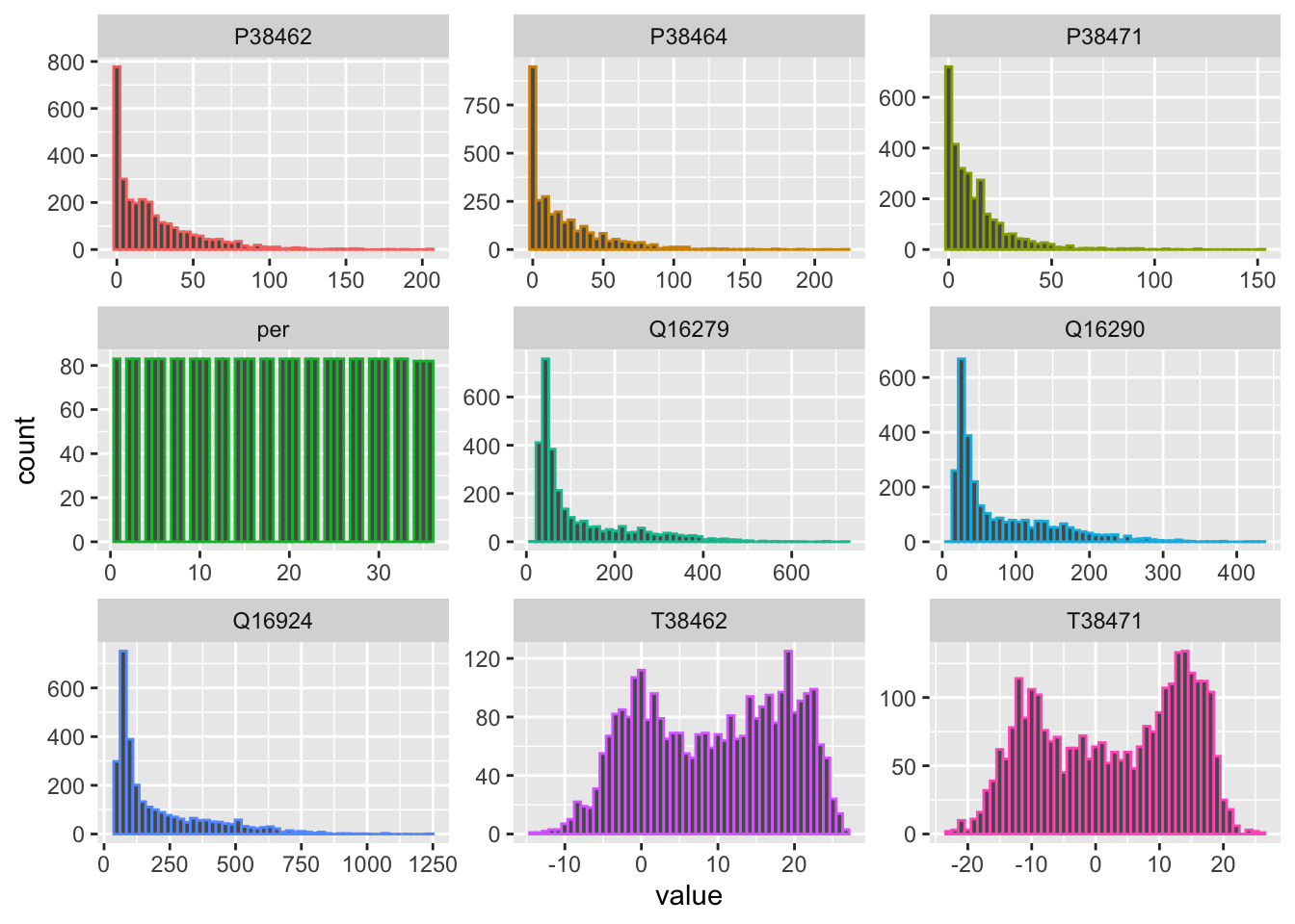
Let us for example look at a very simple uniform non-parametric transformation, i.e. a logarithmic transformation (see Figure 10.13). As compared to parametric transformation, the logarithmic transformation is simple to apply for data greater than zero and does not require us to keep track of transformation parameters as, for example, is the case when we center and scale the data.
data_wide_tbl |>
mutate(across(Q16279:P38471,.fns = log1p)) |> # transforms discharge and precipitation time series
pivot_longer(-date) |>
ggplot(aes(x=value,colour = name)) +
geom_histogram(bins=50) +
facet_wrap(~name, scales = "free") +
theme(legend.position = "none")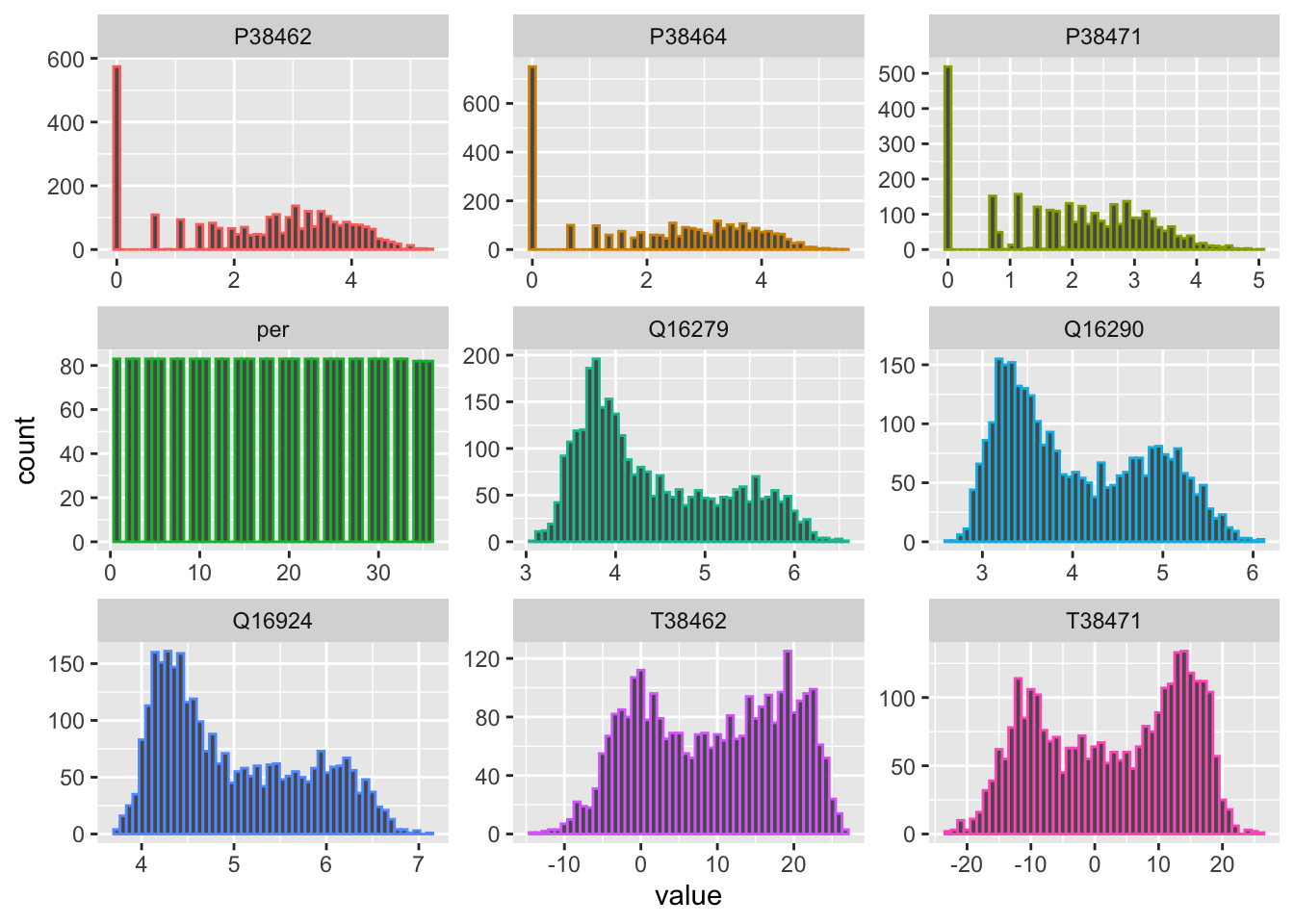
Please note that with the base-R command log1p, 1 is added prior to the logarithmic transformation to avoid cases where the transformed values would not be defined, i.e. where discharge or precipitation is 0. More information about the log1p() function can be obtained by simply typing ?log1p. Recovering the original data after the log1p transformation is simply achieved by taking the exponent of the transformed data and subtracting 1 from the result. The corresponding R function is expm1().
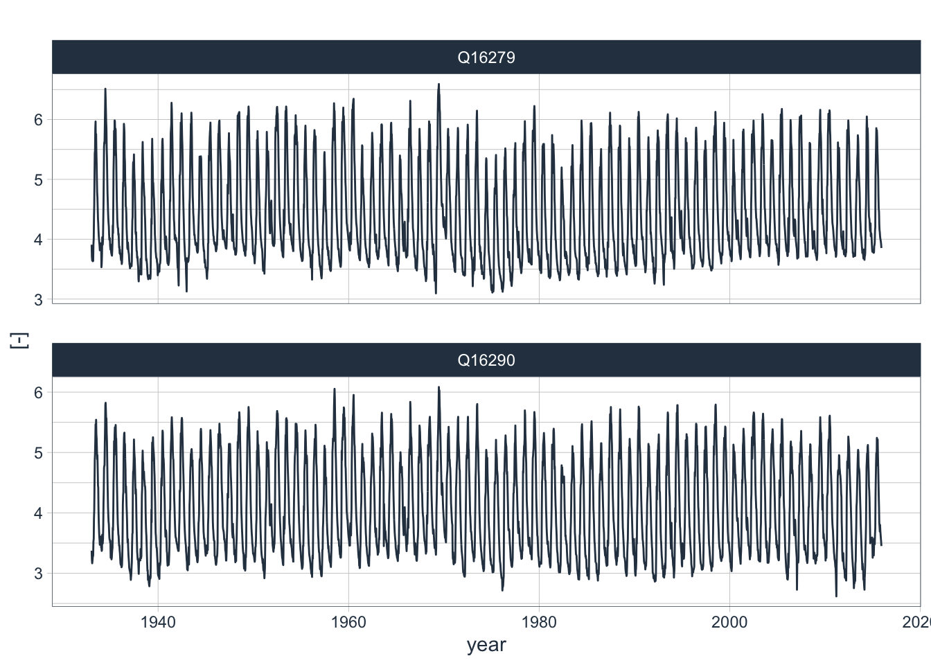
Clearly, the log-transformed discharge values are no longer skewed (Figure @ref(fig:histogramsData_transformed)). We now see interesting bimodal distributions. At the same time, the variance of the transformed variables is greatly reduced. These are two properties that will help us construct a good model as we shall see below. Finally, the transformed discharge time series are shown in Figure .
data_long_tbl |>
filter(name=='Q16279' | name=='Q16290') |>
plot_time_series(date, log(value+1),
.facet_vars = name,
.smooth = FALSE,
.interactive = FALSE,
.title = "",
.y_lab = "[-]",
.x_lab = "year"
)
10.5.2 Detecting Trends
Lower frequency variability in time series, including trends, can be visualized by using the .smooth = TRUE option in the plot_time_series() function. To demonstrate this here, we have a closer look at the temperature data in our data record as shown in Figure 10.15.
data_long_tbl |>
filter(name == 'T38462' | name == 'T38471') |>
plot_time_series(date, value,
.smooth = TRUE,
.facet_vars = name,
.title = "",
.y_lab = "deg. C.",
.x_lab = "year"
)In both time series, a slight upward trend is visible that picks up over the most recent decades. We can look at these trends in greater detail, for example at monthly levels as shown in Figure 10.16.
data_long_tbl |>
filter(name == 'T38462') |>
summarise_by_time(.date_var = date, .by="month",value=mean(value)) |>
tk_ts(frequency = 12) |>
forecast::ggsubseriesplot(year.labels = FALSE) +
geom_smooth(method = "lm",color="red") +
#ggtitle('Development of Monthly Mean Temperatures from 1933 - 2015 at Station 38462') +
xlab('month') +
ylab('Degrees Celsius')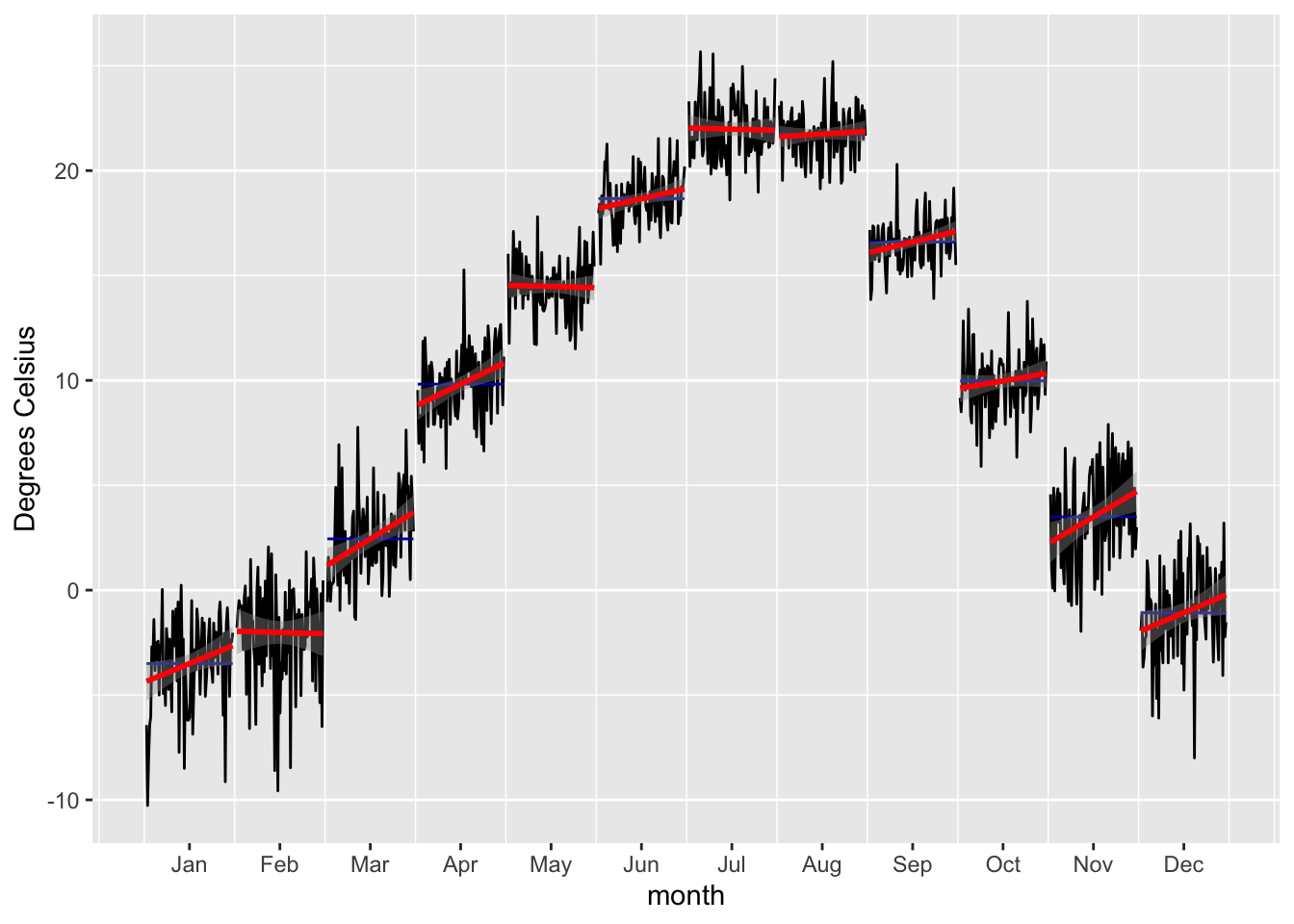
In the Figure above, a significant winter warming over the period of data availability is confirmed at Pskem meteorological station. As discussed in the background Chapters on the Central Asia Hydrological Systems and the Example River Basins, these trends are observed throughout the Central Asian region and are an indication of the changing climate there. We will have to take into account such type of trends in our modeling approach.
10.5.3 Auto- and Cross-Correlations
A time series may have relationships to previous versions of itself - these are the ‘lags’. The autocorrelation is a measure of the strength of this relationship of a series to its lags. The autocorrelation function ACF looks at all possible correlations between observation at different times and how they emerge. Contrary to that, the partial autocorrelation function PACF only looks at the correlation between a particular past observation and the current one. So in other words, ACF includes direct and indirect effects whereas PACF only includes the direct effects between observations at time t and the lag. As we shall see below, PACF is super powerful to identify relevant lagged time series predictors in autoregressive models (AR Models).
Figure 10.17 shows the ACF and PACF over the interval of 72 lags (2 years). The AC function shows the highly seasonal characteristics of the underlying time series. It also shows the pronounced short-term memory in the basin, i.e. the tendency to observe subsequent values of high flows and subsequent values of low flow - hence the smoothness of the curve. This time of autocorrelation behavior is typical for basins with large surface storage in the form of lakes, swamps, snow and glaciers, permafrost and groundwater reserves (A. 2019). The Chatkal river basin certainly belongs to that category.
data_long_tbl |> filter(name == 'Q16279') |>
plot_acf_diagnostics(date, value,
.show_white_noise_bars = TRUE,
.lags = 72,
.title = ""
)But is there also autocorrelation of the annual time series? Let us test.
Q16279_annual <- data_long_tbl |> filter(name == 'Q16279') |> dplyr::select(-name) |>
summarize_by_time(.date_var = date,
.by="year",
sum=sum(value)*3600*24*10/10^9)
Q16279_annual |> plot_time_series(date,sum,
.smooth = FALSE,
.title = "",
.x_lab = "year",
.y_lab = "Discharge [cubic km per year]")Q16279_annual |>
plot_acf_diagnostics(.date_var = date,
.value = sum,
.lags = 50,
.show_white_noise_bars = TRUE,
.title = "",
.x_lab = "year")The ?fig-annual-auto-corr shows a fast decaying autocorrelation function for the annualized time series where even lag 1 values are no longer correlated in a significant manner.
The PAC function, on the other hand, demonstrates that lag 1 is really critical in terms of direct effects (Figure 10.17). After that, the PACF tapers off quickly. To utilize these findings in our modeling approach that uses lagged regression is important, as we shall see below.
We can also study cross-correlations between two different time series. In other words, in cross-correlation analysis between two different time series, we estimate the correlation one variable and another, time-shifted variable. For example, we can cross-correlate discharge at Gauge 16279 (Chatkal river) to discharge at Gauge 16290 (Pskem River) as shown in (fig_cross_corr_q?). As is easily visible, the discharge behavior of the two rivers is highly correlated.
data_wide_tbl |> plot_acf_diagnostics(date,Q16279,
.ccf_vars = Q16290,
.show_ccf_vars_only = TRUE,
.show_white_noise_bars = TRUE,
.lags = 72,
.title = ""
)Cross-correlation analysis of the two discharge time series Q16279 and Q16290.
Converse to this, discharge shows a lagged response to temperature which is clearly visible in the cross-correlation function.
data_wide_tbl |> plot_acf_diagnostics(date,T38471,
.ccf_vars = Q16279,
.show_ccf_vars_only = TRUE,
.show_white_noise_bars = TRUE,
.lags = 72,
.title = ""
)A less pronounced cross-correlation exists between precipitation and discharge when measured at the same stations (Figure @ref(ccf_PQ)).
data_wide_tbl |> plot_acf_diagnostics(date,P38471,
.ccf_vars = Q16279,
.show_ccf_vars_only = TRUE,
.show_white_noise_bars = TRUE,
.lags = 72,
.title = ""
)10.5.4 Time Series Seasonality
There is a pronounced seasonality in the discharge characteristics of Central Asian rivers. One of the key reason of this is the annual melt process of the winter snow pack. Figure 10.22 shows the seasonality of the log-transformed discharge. These observations can help in investigating and detecting time-based (calendar) features that have cyclic or trend effects.
data_long_tbl |>
filter(name=="Q16279" | name=="Q16290") |>
plot_seasonal_diagnostics(date,
log(value+1),
.facet_vars = name,
.feature_set = c("week","month.lbl","year"),
.interactive = FALSE,
.title = ""
)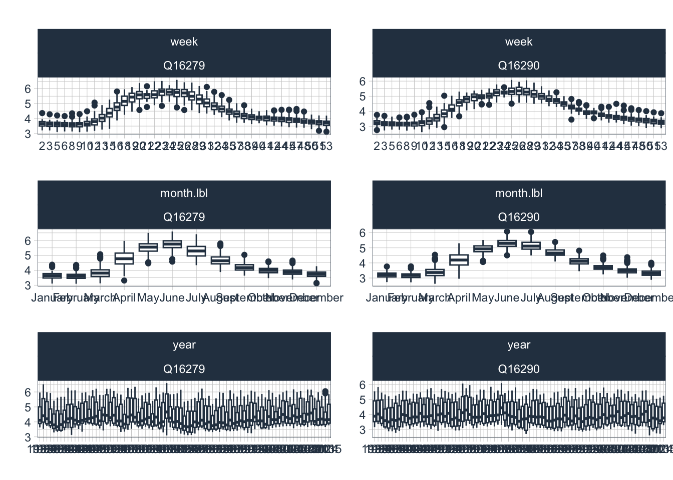
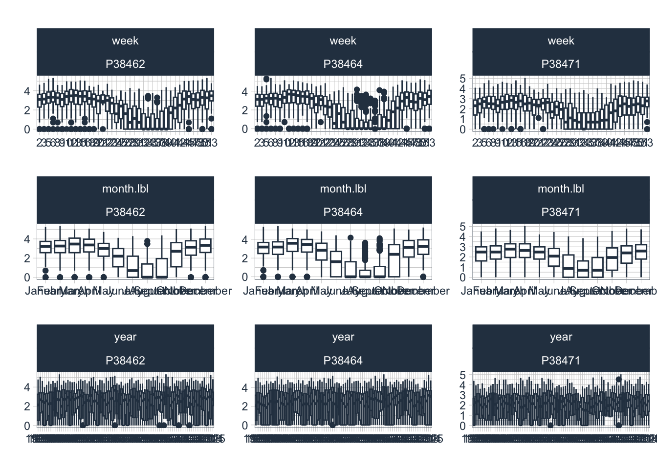
Figure 10.23 shows the seasonal diagnostic for the log-transformed precipitation time series. The significant interannual variability is visible. In the annualized time series, no trend is available.
data_long_tbl |>
filter(name=="P38462" | name=="P38464" | name=="P38471") |>
plot_seasonal_diagnostics(date,
log1p(value),
.facet_vars = name,
.feature_set = c("week","month.lbl","year"),
.interactive = FALSE,
.title = ""
)
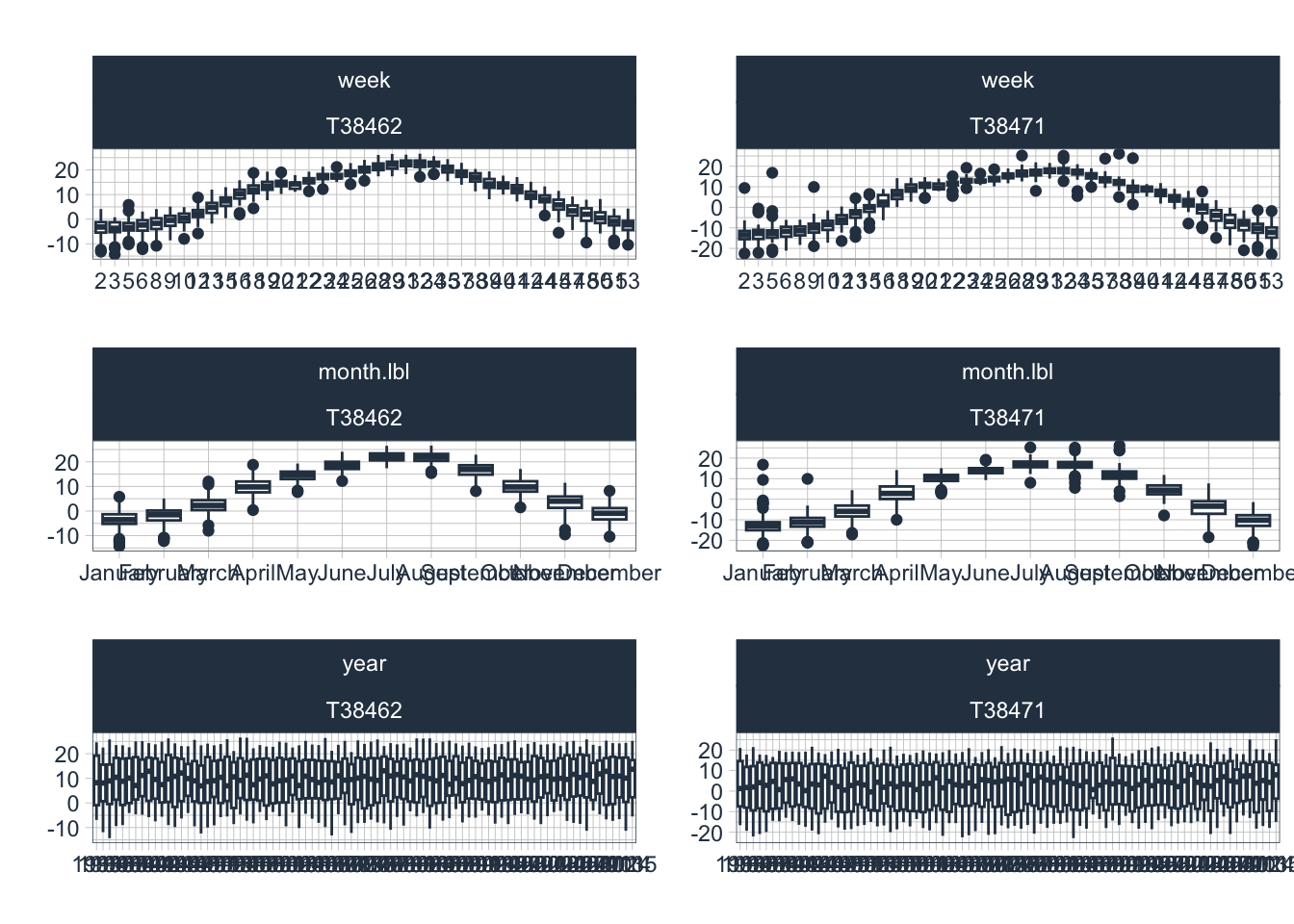
Finally, Figure 10.24 displays the seasonal diagnostics of the temperature time series. Notice that we use untransformed, raw values here for plotting.
data_long_tbl |>
filter(name=="T38462" | name=="T38471") |>
plot_seasonal_diagnostics(date,
value,
.facet_vars = name,
.feature_set = c("week","month.lbl","year"),
.interactive = FALSE,
.title = "",
)
10.6 Investigating and Engineering Predictors
All the data that we have available have been analyzed by now and we can now move to generating a good and solid understanding of the relevance of predictors for statistical modeling. To start with, we will keep things deliberately simple. Our approach is tailored to the particular local circumstances and the needs and wants of the hydrometeorological agencies that are using such types of model to issue high quality forecasts.
First, the plan here to start with the introduction and discussion of the current forecasting techniques that are used operationally inside the Kyrgyz Hydrometeorological agency. These models and their forecast quality will serve as benchmark to beat any of the other models introduced here. At the same time, we will introduce a measure with which to judge forecast quality.
Secondly, we evaluate the simplest linear models using time series regression. This will also help to introduce and explain key concepts that will be discussed in the third and final section below.
Finally, we show the application of more advanced forecasting modeling techniques that use state-of-the-art regression type algorithms.
The forecasting techniques will be demonstrated by focussing on the Pskem river. The techniques extend to other rivers in the region and beyond in a straight forward manner.
10.6.1 Benchmark: Current Operational Forecasting Models in the Hydrometeorological Agencies
More information to come. Check back soon here.
10.6.2 Time Series Regression Models
The simplest linear regression model can be written as
\[ y_{t} = \beta_{0} + \beta_{1} x_{t} + \epsilon_{t} \]
where the coefficient \(\beta_{0}\) is the intercept term, \(\beta_{1}\) is the slope and \(\epsilon_{t}\) is the error term. The subscripts \(t\) denote the time dependency of the target and the explanatory variables and the error. \(y_{t}\) is our target variable, i.e. discharge in our case, that we want to forecast. At the same time, \(x_{t}\) is an explanatory variable that is already observed at time \(t\) and that we can use for prediction.
As we shall see below, we are not limited to the inclusion of only one explanatory variable but can think of adding multiple variables that we suspect to help improve forecast modeling performance.
To demonstrate the effects of different explanatory variables on our forcasting target and the quality of our model for forecasting discharge at stations 16290, the function plot_time_series_regression from the timetk package is used. First, we we only want to specify a model with a trend over the time \(t\). Hence, we fit the model
\[ y_{t} = \beta_{0} + \beta_{1} t + \epsilon_{t} \]
model_formula <- as.formula(log1p(Q16290) ~
as.numeric(date)
)
model_data <- data_wide_tbl |> dplyr::select(date,Q16290)
model_data |>
plot_time_series_regression(
.date_var = date,
.formula = model_formula,
.show_summary = TRUE,
.title = ""
)
Call:
stats::lm(formula = .formula, data = df)
Residuals:
Min 1Q Median 3Q Max
-1.3940 -0.7068 -0.2114 0.7193 2.0274
Coefficients:
Estimate Std. Error t value Pr(>|t|)
(Intercept) 4.056e+00 1.489e-02 272.39 <2e-16 ***
as.numeric(date) -2.997e-06 1.675e-06 -1.79 0.0736 .
---
Signif. codes: 0 '***' 0.001 '**' 0.01 '*' 0.05 '.' 0.1 ' ' 1
Residual standard error: 0.7998 on 2983 degrees of freedom
Multiple R-squared: 0.001073, Adjusted R-squared: 0.0007378
F-statistic: 3.203 on 1 and 2983 DF, p-value: 0.07359Note that the timetk::plot_time_series function is a convenience wrapper to make our lives easy in terms of modeling and immediately getting a resulting plot. The same model could be specified in the traditional R-way, i.e. as follows
Call:
lm(formula = model_formula, data = model_data)
Residuals:
Min 1Q Median 3Q Max
-1.3940 -0.7068 -0.2114 0.7193 2.0274
Coefficients:
Estimate Std. Error t value Pr(>|t|)
(Intercept) 4.056e+00 1.489e-02 272.39 <2e-16 ***
as.numeric(date) -2.997e-06 1.675e-06 -1.79 0.0736 .
---
Signif. codes: 0 '***' 0.001 '**' 0.01 '*' 0.05 '.' 0.1 ' ' 1
Residual standard error: 0.7998 on 2983 degrees of freedom
Multiple R-squared: 0.001073, Adjusted R-squared: 0.0007378
F-statistic: 3.203 on 1 and 2983 DF, p-value: 0.07359The adjusted R-squared shows the mediocre performance of our simple model as it cannot capture any of the seasonal variability. Furthermore we see that the trend coefficient is negative which indicates a decrease in mean discharge. However, as the p-value confirms, the trend is only significant at the 0.1 level.
The first step in improving our model is to account for seasonality. In the case of decadal time series, we can add categorical variables (as factor variables) decoding the corresponding decades. Similarly, in the case of monthly data, we could use month names or factors 1..12 to achieve the same. The same reasoning extends to other periods (quarters, weekdays, etc.). We will use a quarterly model to explain the concept since the inclusion of 4 indicator variables for the individual quarters is easier to grasp than to work with 36 decadal indicators.
# Computing quarterly mean discharge values
q16290_quarter_tbl <- model_data |>
summarize_by_time(date,value=mean(log1p(Q16290)),.by = "quarter")
# adding quarters identifier
q16290_quarter_tbl <- q16290_quarter_tbl |>
mutate(per = quarter(date) |> as.factor())
model_formula <- as.formula(value ~
as.numeric(date) +
per
)
q16290_quarter_tbl |>
plot_time_series_regression(date,
.formula = model_formula,
.show_summary = TRUE,
.title = ""
)
Call:
stats::lm(formula = .formula, data = df)
Residuals:
Min 1Q Median 3Q Max
-0.51477 -0.14936 0.00228 0.14410 0.66161
Coefficients:
Estimate Std. Error t value Pr(>|t|)
(Intercept) 3.255e+00 2.204e-02 147.691 < 2e-16 ***
as.numeric(date) -3.158e-06 1.255e-06 -2.516 0.0123 *
per2 1.551e+00 3.106e-02 49.919 < 2e-16 ***
per3 1.396e+00 3.107e-02 44.938 < 2e-16 ***
per4 2.562e-01 3.107e-02 8.248 3.98e-15 ***
---
Signif. codes: 0 '***' 0.001 '**' 0.01 '*' 0.05 '.' 0.1 ' ' 1
Residual standard error: 0.2001 on 327 degrees of freedom
Multiple R-squared: 0.9217, Adjusted R-squared: 0.9207
F-statistic: 962.4 on 4 and 327 DF, p-value: < 2.2e-16What we did here is to compare a continuous variable, i.e. the discharge, across 4 categories. Hence, we can write down the model in the following way:
\[ y_{t} = \beta_{0} + \beta_{1} \delta_{t}^{Qtr2} + \beta_{2} \delta_{t}^{Qtr3} + \beta_{3} \delta_{t}^{Qtr4} + \epsilon_{t} \]
Using ‘one hot encoding’, we include only N-1 (here, 3) variables out of the N (here,4) in the regression because we can safely assume that if we are in Quarter 4, all the other indicator variables are simply 0. If we are in quarter 1 (Qtr1), the model would just be
\[ y_{t} = \beta_{0} + \epsilon_{t} \]
If we are in Quarter 2 (Qtr2), the model would be
\[ y_{t} = \beta_{0} + \beta_{1} + \epsilon_{t} \]
since \(\delta_{t}^{Qtr2} = 1\). Hence, whereas \(\beta_{0}\) is to be interpreted as the estimated mean discharge in Quarter 1 (called (Intercept) in the results table below), \(\beta_{1}\) (called qtr2 in the results table below) is the estimated difference of mean discharge between the two categories/quarters We can get the values and confidence intervals of the estimates easily in the following way
lm_quarterlyModel <- q16290_quarter_tbl |>
lm(formula = model_formula)
meanQtrEstimates <- lm_quarterlyModel |> coefficients()
meanQtrEstimates |> expm1() (Intercept) as.numeric(date) per2 per3
2.493125e+01 -3.158103e-06 3.714894e+00 3.039112e+00
per4
2.920533e-01 2.5 % 97.5 %
(Intercept) 2.383084e+01 2.608043e+01
as.numeric(date) -5.627148e-06 -6.890525e-07
per2 3.435387e+00 4.012016e+00
per3 2.799662e+00 3.293653e+00
per4 2.154539e-01 3.734800e-01The same reasoning holds true for the model with decadal observations to which we return now again. First, we add decades as factors to our data_wide_tbl.
Now, we can specify and calculate the new model.
model_formula <- as.formula(log1p(Q16290) ~
as.numeric(date) + # trend components
per # seasonality (as.factor)
)
model_data <- data_wide_tbl |> dplyr::select(date,Q16290,per)
model_data |>
plot_time_series_regression(
.date_var = date,
.formula = model_formula,
.show_summary = TRUE,
.title = ""
)
Call:
stats::lm(formula = .formula, data = df)
Residuals:
Min 1Q Median 3Q Max
-1.3225 -0.6972 -0.2318 0.7268 2.0364
Coefficients:
Estimate Std. Error t value Pr(>|t|)
(Intercept) 3.943e+00 2.991e-02 131.827 < 2e-16 ***
as.numeric(date) -3.065e-06 1.670e-06 -1.836 0.0665 .
per 6.150e-03 1.406e-03 4.374 1.26e-05 ***
---
Signif. codes: 0 '***' 0.001 '**' 0.01 '*' 0.05 '.' 0.1 ' ' 1
Residual standard error: 0.7974 on 2982 degrees of freedom
Multiple R-squared: 0.00744, Adjusted R-squared: 0.006774
F-statistic: 11.18 on 2 and 2982 DF, p-value: 1.46e-05What we see is that through the inclusion of the categorical decade variables, we have greatly improved our modeling results since we can now capture the seasonality very well (Tip: zoom into the time series to compare highs and lows and their timing for the target variable and its forecast). However, despite the excellent adjusted R-squared value of 0.9117, our model is far from perfect as it is not able to account for inter-annual variability in any way.
Let us quickly glance at the errors.
#} fig-cap: "Scatterplot of observed versus calculated values."
lm_decadalModel <- model_data |>
lm(formula = model_formula)
obs_pred_wide_tbl <- model_data|>
mutate(pred_Q16290 = predict(lm_decadalModel) |> expm1()) |>
mutate(error = Q16290 - pred_Q16290)
ggplot(obs_pred_wide_tbl, aes(x = Q16290,
y = pred_Q16290,
colour = per )) +
geom_point() +
geom_abline(intercept = 0, slope = 1)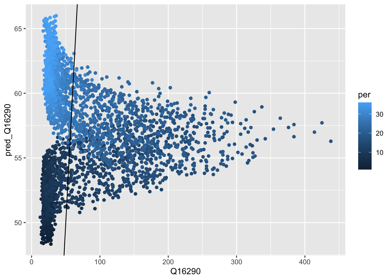
We do not seem to make a systematic error as also confirmed by inspecting the histogram or errors (they are nicely centered around 0).
ggplot(obs_pred_wide_tbl,aes(x=error)) +
geom_histogram(bins=100)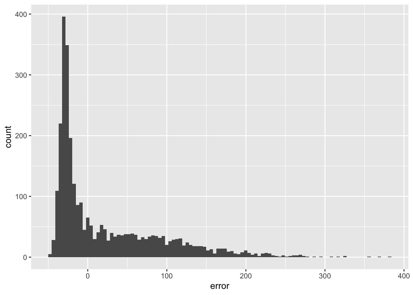
In Section 10.5.3 above, we saw that the PAC function is very high at lag 1. We exploit this fact be incorporating in the regression equation the observed previous discharge, i.e. \(y_{t-1}\) at time \(t-1\) to predict discharge at time \(t\). Hence, our regression can be written as
\[ y_{t} = \beta_{0} + \beta_{1} t + \beta_{2} y_{t-1} + \sum_{j=2}^{36} \beta_{j} \delta_{t}^{j} + \epsilon_{t} \]
where the \(\delta_t^{j}\) correspondingly are the 35 indicator variables as discussed above in the case of quarterly time series where we had 3 of these variables included. Before we can estimate this model, we prepare a tibble with the relevant data as shown in the table below (note that we simply renamed the discharge column to Q out of convenience).
model_data <- data_wide_tbl |>
dplyr::select(date,Q16290,per) |>
rename(Q=Q16290) |>
mutate(Q = log1p(Q)) |>
mutate(Q_lag1 = lag(Q,1))
model_data# A tibble: 2,985 × 4
date Q per Q_lag1
<date> <dbl> <int> <dbl>
1 1933-01-10 3.37 1 NA
2 1933-01-20 3.23 2 3.37
3 1933-01-31 3.17 3 3.23
4 1933-02-10 3.21 4 3.17
5 1933-02-20 3.26 5 3.21
6 1933-02-28 3.28 6 3.26
7 1933-03-10 3.30 7 3.28
8 1933-03-20 3.53 8 3.30
9 1933-03-31 3.57 9 3.53
10 1933-04-10 3.92 10 3.57
# ℹ 2,975 more rowsNotice that to accommodate the \(y_{t-1}\) in the data, we simply add a column that contains a lagged version of the discharge time series itself (see column Q_lag1). Now, for example, for our regression we have a first complete set of data points on \(t = '1933-01-20'\), with \(Q=3.226844\), \(dec=2\) and \(Q_{lag1}=3.374169\). Notice how the last value corresponds to the previously observed and now known \(y_{t-1}\).
# Specification of the model formula
model_formula <- as.formula(Q ~ as.numeric(date) + per + Q_lag1)
# Note that we use na.omit() to delete incomplete data records, ie. the first observation where we lack the lagged value of the discharge.
model_data |> na.omit() |> lm(formula = model_formula) |> summary()
Call:
lm(formula = model_formula, data = na.omit(model_data))
Residuals:
Min 1Q Median 3Q Max
-1.09294 -0.12965 -0.03140 0.07656 1.17980
Coefficients:
Estimate Std. Error t value Pr(>|t|)
(Intercept) 1.955e-01 1.801e-02 10.850 <2e-16 ***
as.numeric(date) -6.402e-08 3.925e-07 -0.163 0.87
per -7.010e-03 3.355e-04 -20.897 <2e-16 ***
Q_lag1 9.838e-01 4.353e-03 225.992 <2e-16 ***
---
Signif. codes: 0 '***' 0.001 '**' 0.01 '*' 0.05 '.' 0.1 ' ' 1
Residual standard error: 0.1873 on 2980 degrees of freedom
Multiple R-squared: 0.9453, Adjusted R-squared: 0.9452
F-statistic: 1.716e+04 on 3 and 2980 DF, p-value: < 2.2e-16It looks like we have made a decisive step in the right direction by incorporating the previously observed discharge value. Also, notice that some of the decade factors have lost their statistical significance meaning that the seasonality can now be captured in part also by the lagged version of the time series.
Let us visualize the results quickly (tip: also zoom in to explore the fit).
model_data |>
na.omit() |>
plot_time_series_regression(
.date_var = date,
.formula = model_formula,
.show_summary = FALSE, # We do show the summary since we have plotted the summary output already above.
.title = ""
)This is clearly an astonishing result. Nevertheless, we should keep a couple of things in mind:
- What about the rate of change of the discharge and the acceleration of discharge? Would the incorporation of these features help to improve the model?
- We have not assess the quality of the forecasts using the stringent quality criteria as they exist in the Central Asian Hydrometeorological Services. How does our forecast perform under this criteria?
- Does the incorporation of precipitation and temperature data help to improve our forecast skills?
- We did not test our model on out-of-sample data. Maybe our model does not generalize well? We will discuss these and related issues soon when using more advanced models but for the time being declare this a benchmark model due to its simplicity and predictive power.
We will work on these questions now and focus first on the incorporation of the rate of change in discharge and the acceleration of discharge over time. First, we add \(Q_{lag2}\) to our model data and then compute change and acceleration accordingly.
model_data <- model_data |>
mutate(Q_lag2 = lag(Q,2)) |>
mutate(change = Q_lag1 -Q_lag2) |> # that is the speed of change in discharge
mutate(change_lag1 = lag(change,1)) |>
mutate(acc = change - change_lag1) |> na.omit() # and that is the acceleration of discharge
model_data# A tibble: 2,982 × 8
date Q per Q_lag1 Q_lag2 change change_lag1 acc
<date> <dbl> <int> <dbl> <dbl> <dbl> <dbl> <dbl>
1 1933-02-10 3.21 4 3.17 3.23 -0.0614 -0.147 0.0860
2 1933-02-20 3.26 5 3.21 3.17 0.0413 -0.0614 0.103
3 1933-02-28 3.28 6 3.26 3.21 0.0551 0.0413 0.0138
4 1933-03-10 3.30 7 3.28 3.26 0.0152 0.0551 -0.0399
5 1933-03-20 3.53 8 3.30 3.28 0.0187 0.0152 0.00348
6 1933-03-31 3.57 9 3.53 3.30 0.231 0.0187 0.212
7 1933-04-10 3.92 10 3.57 3.53 0.0432 0.231 -0.187
8 1933-04-20 4.05 11 3.92 3.57 0.348 0.0432 0.305
9 1933-04-30 4.47 12 4.05 3.92 0.132 0.348 -0.216
10 1933-05-10 4.88 13 4.47 4.05 0.416 0.132 0.284
# ℹ 2,972 more rows# Specification of the model formula
model_formula <- as.formula(Q ~ as.numeric(date) + per + Q_lag1 + change + acc)
model_data |> na.omit() |>
plot_time_series_regression(
.date_var = date,
.formula = model_formula,
.show_summary = TRUE, # We do show the summary since we have plotted the summary output already above.
.title = ""
)
Call:
stats::lm(formula = .formula, data = df)
Residuals:
Min 1Q Median 3Q Max
-1.01892 -0.09223 -0.02294 0.05501 1.16531
Coefficients:
Estimate Std. Error t value Pr(>|t|)
(Intercept) 2.574e-01 1.626e-02 15.830 <2e-16 ***
as.numeric(date) -1.834e-07 3.480e-07 -0.527 0.598
per -2.859e-03 3.318e-04 -8.616 <2e-16 ***
Q_lag1 9.496e-01 4.087e-03 232.331 <2e-16 ***
change 5.650e-01 2.002e-02 28.221 <2e-16 ***
acc -2.215e-01 1.806e-02 -12.265 <2e-16 ***
---
Signif. codes: 0 '***' 0.001 '**' 0.01 '*' 0.05 '.' 0.1 ' ' 1
Residual standard error: 0.1658 on 2976 degrees of freedom
Multiple R-squared: 0.9571, Adjusted R-squared: 0.957
F-statistic: 1.328e+04 on 5 and 2976 DF, p-value: < 2.2e-16
Call:
lm(formula = model_formula, data = model_data)
Residuals:
Min 1Q Median 3Q Max
-1.01892 -0.09223 -0.02294 0.05501 1.16531
Coefficients:
Estimate Std. Error t value Pr(>|t|)
(Intercept) 2.574e-01 1.626e-02 15.830 <2e-16 ***
as.numeric(date) -1.834e-07 3.480e-07 -0.527 0.598
per -2.859e-03 3.318e-04 -8.616 <2e-16 ***
Q_lag1 9.496e-01 4.087e-03 232.331 <2e-16 ***
change 5.650e-01 2.002e-02 28.221 <2e-16 ***
acc -2.215e-01 1.806e-02 -12.265 <2e-16 ***
---
Signif. codes: 0 '***' 0.001 '**' 0.01 '*' 0.05 '.' 0.1 ' ' 1
Residual standard error: 0.1658 on 2976 degrees of freedom
Multiple R-squared: 0.9571, Adjusted R-squared: 0.957
F-statistic: 1.328e+04 on 5 and 2976 DF, p-value: < 2.2e-16# Here, we add the the prediction to our tibble so that we can assess model predictive quality later.
model_fc_wide_tbl <- model_data |>
mutate(pred = predict(model)) |>
mutate(obs = expm1(Q), pred = expm1(pred)) |>
dplyr::select(date,obs,pred,per)
model_fc_wide_tbl# A tibble: 2,982 × 4
date obs pred per
<date> <dbl> <dbl> <int>
1 1933-02-10 23.7 23.6 4
2 1933-02-20 25.1 25.9 5
3 1933-02-28 25.5 28.0 6
4 1933-03-10 26 28.1 7
5 1933-03-20 33 28.3 8
6 1933-03-31 34.5 38.1 9
7 1933-04-10 49.3 38.9 10
8 1933-04-20 56.4 58.0 11
9 1933-04-30 86 65.3 12
10 1933-05-10 130 102. 13
# ℹ 2,972 more rowsAnother, albeit small improvement in the forecast of predicting discharge 1-step ahead! It is now time to properly gauge the quality of this seemingly excellent model. Does it conform to local quality standards that apply to decadal forecasts? The Figure 10.30 shows the un-transformed data. We see that we are not doing so well during the summer peak flows. As we shall see further below, these are the notoriously hard to predict values, even just for 1-step ahead decadal predictions.
model_fc_wide_tbl |>
dplyr::select(-per) |>
pivot_longer(-date) |>
plot_time_series(date,
value,
name,
.smooth = F,
.title = "")10.6.3 Assessing the Quality of Forecasts
How well are we doing with our simple linear model? Let us assess the model quality using the local practices. For the Central Asian Hydromets, a forecast at a particular decade \(d\) is considered to be excellent if the following holds true
\[ |Q_{obs}(d,y) - Q_{pred}(d,y)| \le 0.674 \cdot \sigma[\Delta Q(d)] \]
where \(Q_{obs}(d,y)\) is the observed discharge at decade \(d\) and year \(d\), \(Q_{pred}(d,y)\) is the predicted discharge at decade \(d\) and year \(y\), \(|Q_{obs}(d) - Q_{pred}(d)|\) thus the absolute error and \(\sigma[\Delta Q(d)] = \sigma[Q(d) - Q(d-1)]\) is the standard deviation of the difference of decadal observations at decade \(d\) and \(d-1\) over the entire observation record (hence, the year indicator \(y\) is omitted there). The equation above can be reformulated to
\[ \frac{|Q_{obs}(d,y) - Q_{pred}(d,y)|}{\sigma[\Delta Q(d)]} \le 0.674 \]
So let us assess the forecast performance over the entire record using the `riversCentralAsia::assess_fc_qual`` function. Note that the function returns a list of three objects. First, it returns a tibble of the number of forecasts that are of acceptable quality for the corresponding period (i.e. decade or month) as a percentage of the total number of observations that are available for that particular period. Second, it returns the period-averaged mean and third a figure that shows forecast quality in two panels.
So, for our model which we consiedered to be performing well above, we get the following performance specs
plot01 <- TRUE
te <- assess_fc_qual(model_fc_wide_tbl,plot01)
te[[3]]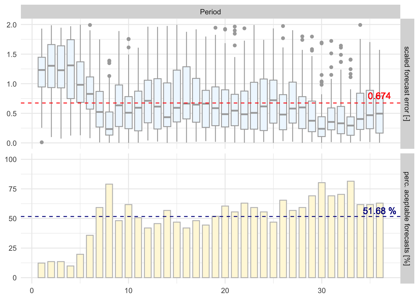
In other words, roughly two thirds of our in-sample forecasts comply will be considered good enough when measured according to the quality criterion. Furthermore, the model performs worse than average during the second quarter (Q2) decades, i.e. from decade 10 through 17. This is an indication that providing good forecasts in Q2 might be hard.
It is, however, generally not considered to be good practice to assess model quality on in-sample data. Rather, model performance should be assessed on out-of-sample data that was not used for model training and is thus data that is entirely unseen.
10.6.4 Generating and Assessing Out-of-Sample Forecasts
Note, this Section is work in progress. Please check back later!
We start off with our model_data tibble and want to divide it into two sets, one for model training and one for model testing. We refer to these sets as training set and test set. For the creation of these sets, we can use the timetk::time_series_split() function.
10.6.5 Machine Learning Models
Note, this Section is work in progress. Please check back later!