12 Quantification of Climate Change Impacts
Here, we describe conducting a climate change impact study in a gauged catchment from scratch. With much of the background information and the data already provided in Parts I and II of this Handbook, the focus is to provide a concise and easy-to-follow step-by-step guide.
We will use the Zarafshan River Basin as an example. The Zarafshan River Basin is shared between upstream Tajikistan and downstream Uzbekistan and is part of the larger Amu Darya River Basin. The basin is vulnerable to climate change, as is shown here. The Zarafshan River Basin is a typical example of a Central Asia basin. The methods and tools used in this chapter can be applied to other basins in Central Asia and beyond.
Each Section of the Climate Impact Study is structured similarly and contains a Theory Section followed by an Exercise Section. The Theory Section provides a short introduction and theoretical background to each topic. The Exercise section is a step-by-step guide through all the working steps on how to carry out a climate impact study, with the example of the Zarafshan River Basin. This section is supported by tutorial videos in Russian and English and hosted on the HSOL YouTube channel.
We will start with GIS-related work, including watershed delineation, characterization, and the definition of hydrological response units. Then, we move to climate forcing data and their preparation, including historical climate forcing data and climate data using GCM simulations for different CMIP6 scenario pathways. The data are prepared and bias-corrected for all hydrological response units. The implementation, calibration, and validation of the baseline hydrological model are then shown. This is followed by calculating and analyzing the climate scenarios and quantifying the impacts.
The usual prerequisites as for the other Chapters exist. These include access to a computer with the following software installed:
- R: free and open-source statistical programming language
- QGIS: free and open-source Geographical Information System (GIS)
- RS Minerve: Hydrological modeling
Please refer to Section 1.1 to find links for installing the required software. Additional support is also provided in Section A.2, Section A.3, and Section A.3.2.
12.1 Watershed Delineation
In this chapter, we examine the definition of a watershed and how it is delineated using a Geographic Information System (GIS) and a Digital Elevation Model (DEM). We also explore the basics of GIS and the concept of a DEM.
12.1.1 Definition of a Watershed
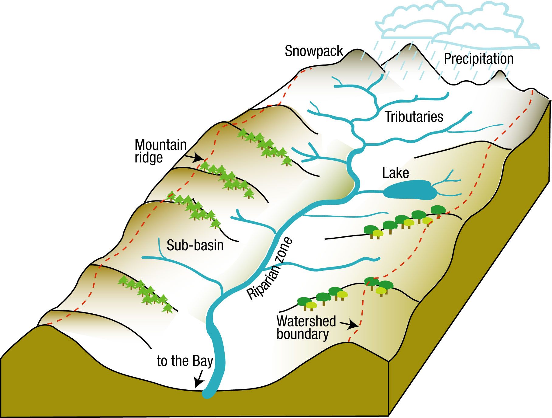
A watershed, often also referred to as a catchment or drainage basin, is a landscape unit over which the hydrological balance can be determined (measured or computed). It is the area draining to a common point. Watershed delineation is creating a boundary representing the contributing area for a particular point/outlet. The topography is the main driving force behind watershed delineation. To find the watershed boundary, we need to pick a point (outlet) and find the area draining into it. We do this to select properties within the watershed, as well as the climate forcing.
In hydrological modeling, we basically compute the water balance for the watershed. The water balance is the difference between the inputs and outputs of water in the system and the resulting change in storage. The water balance equation is given by:
\[ P + SM - ET - I- Q = 0 \tag{12.1}\]
Where \(P\) is the precipitation, \(SM\) snowmelt, \(ET\) evapotranspiration, \(I\) infiltration and \(Q\) the discharge.
12.1.2 Geographic Information System (GIS)
We perform all operations in a Geographic Information System (GIS). A GIS allows us to manage, analyse, edit, produce, and visualise geographic data, also known as spatial data. This is data that includes additional location information. Spatial data comes in two forms: vector and raster data.
Vector points are simply X,Y coordinates and can represent a location like a discharge station, for example. A vector line is a connected sequence of points (e. g. river, street). A vector polygon is a closed set of lines, like a watershed boundary.
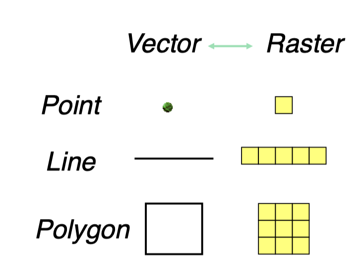
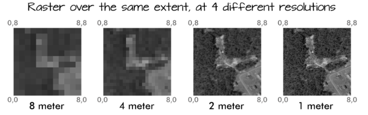
Raster data is made up of pixels (also referred to as grid cells). They are usually regularly spaced and square but don’t have to be. Each pixel is associated with a specific geographical location. Examples of raster data are land use and elevation data. The spatial resolution of raster data refers to the cell geometry, how “big” one cell is. Figure 12.3 shows the effect of different spatial resolutions.
12.1.3 Coordinate Reference System (CRS)
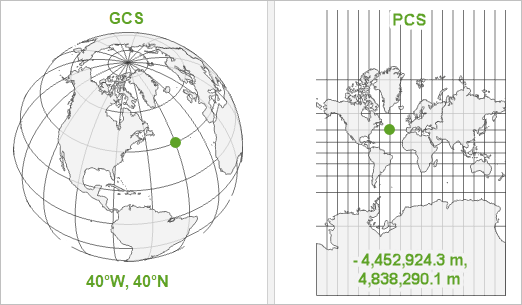
To define the location of objects on the Earth you need a coordinate reference system that adapts to the Earth’s shape. There are two different types of a Coordinate Reference Systems (CRS):
A Geographic coordinate systems (GCS) is a system that uses a three-dimensional spherical surface to determine locations on the Earth. Any location on Earth can be referenced by a point with longitude and latitude coordinates. Its units are angular, usually degrees. (Figure 12.4, right)
A Projected coordinate system (PCS) is flat. It contains a GCS, but it converts that GCS into a flat surface by projecting points into the plane. Its units are linear, for example, in meters Figure 12.4, left)
There are many different models of the earth’s surface, and therefore many different GCS. World Geodetic System 1984 (WGS84) is designed as a one-size-fits-all GCS, good for mapping global data and the most popular CRS. WGS84 uses a three-dimensional ellipsoidal model of the Earth, with positions that are defined using latitude and longitude in degree (e.g. Location of Zurich: E: 47.4°, N: 8.5°).
The Universal Transverse Mercator (UTM) system is a commonly used projected coordinate reference system, in meter. UTM subdivides the globe into zones, numbered 0-60 (equivalent to longitude) and regions (north and south). A UTM zone is a 6° segment of the Earth. Because a circle has 360°, this means that there are 60 UTM zones on Earth. The coordinate system grid for each zone is projected individually. Additionally, the system includes a series of horizontal bands, each covering 8 degrees of latitude, which are lettered from C to X. Zurich, for example, is in UTM zone 32T with the location: 32T E: 465207.85 N: 5246235.11.
12.1.4 Digital Elevation Model (DEM)
A Digital Elevation Model (DEM) represents the Earth’s bare ground topographic surface, excluding trees, buildings, and any other surface objects. There are several datasets available. This handbook will use the digital elevation model from the Shuttle Radar Topography Mission (SRTM) (“NASA Shuttle Radar Topography Mission (SRTM)” (2013)). There are several ways to download the data. This will be discussed within the exercise (?sec-basin-characterisation-exercise-Part1).
12.1.5 Watershed Delineation
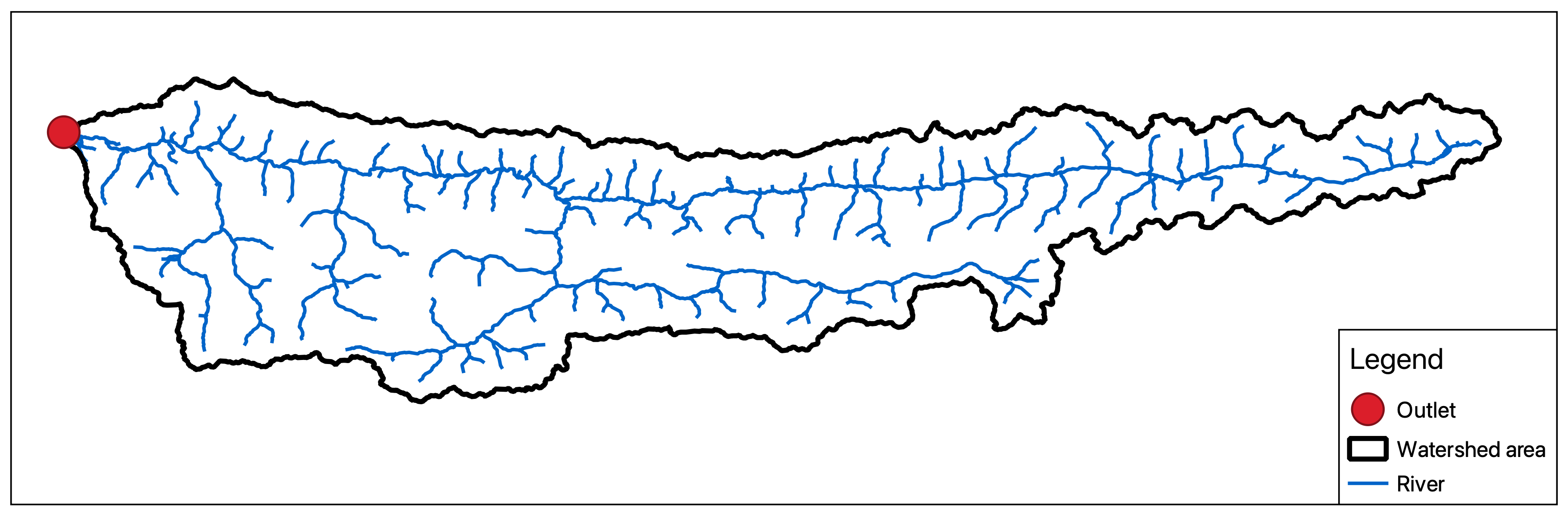
Watersheds can be delineated from a DEM. In this Coursebook, we look at the point-based watershed delineation. The point-based method derives a watershed for each selected point (e.g. discharge station). The slideshow below shows the steps to delineate a watershed based on the example of the upper Zarafshan River Basin.
The outlet point of a watershed is where all the water drains into. Water flow is mainly driven by gravity. From a DEM, we are getting information about the height structure of the surface. To delineate a watershed, first, we have to fill in sinks. A filled DEM is void of depressions, cells that are surrounded by higher elevation values and thus represent an area of internal drainage. From the filled DEM, we can calculate the flow direction. The flow direction shows the direction in which the water will flow out of each cell of the filled DEM. A widely used method for deriving flow direction is the D8 method. The D8 method assigns a cell’s flow direction based on the steepest slope of its eight neighbours. From the flow direction, we can calculate the flow accumulation of each cell by counting how many cells are draining into one cell. The stream network can be derived from a flow accumulation raster by, for example, using a threshold method. This means if a cell of the flow accumulation raster exceeds a certain threshold of how many cells are draining into this cell, it is classified as a river.
Exercise 1: Watershed delineation
The goal of the first exercise is to delineate the catchment, like in the example of upper ZRB in Figure Figure 12.5. For this exercise, you need to have QGIS installed. For a quick installation guide and tutorial, follow this Link. If you already have your catchment outlines and river network, you can skip this exercise and go to sec-basin-characterisation-theory.
In this exercise, we will use the Global Watersheds web app by Heberger (2022). The following instruction video shows how to delineate the catchment and import your watershed area and river network into QGIS.
English version:
Russian version:
Watershed delineation can also be performed using other tools such as QGIS, detailed in Chapter Section 5.2, or R, as outlined here.
12.2 Watershed Characterization
12.2.1 Land Use and Land Cover
In hydrological modeling, we are transforming rainfall into a runoff called rainfall-runoff transformation. When precipitation reaches the ground it can take various pathways. It can be stored as ice or snow, directly evaporate, infiltrate into the ground etc.
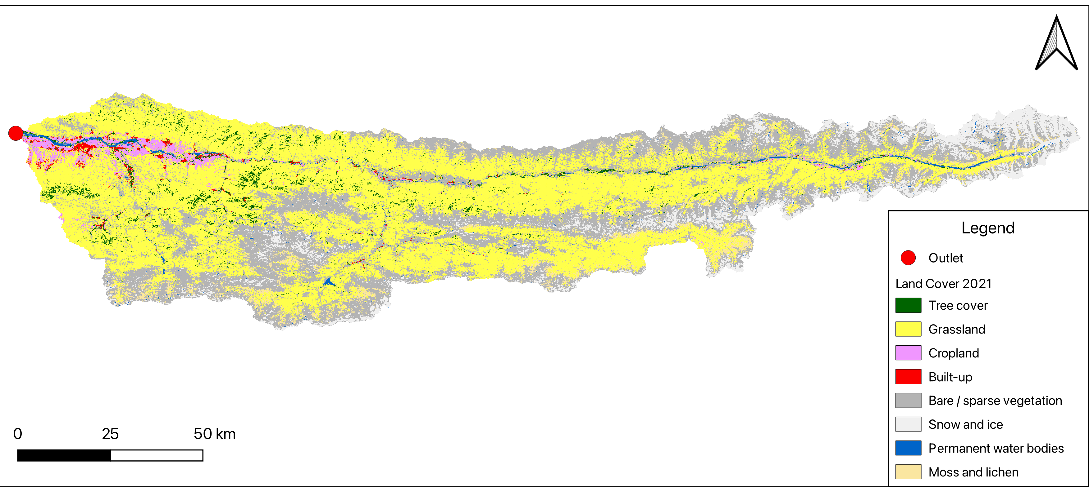
Land cover (LC) maps represent spatial information on different types (classes) of physical coverage of the Earth’s surface, e.g. forests, grasslands, croplands, lakes, wetlands.
The land cover is a key influencer for runoff generation and the estimation of evapotranspiration in the hydrology of watersheds. Therefore, it is essential to use accurate and reliable LC data in hydrological modelling.
Several datasets are available globally and free of charge. Below is a brief list of the most recent land cover data products:
WorldCover project, part of the European Space Agency’s Earth observation program provides global land cover products for 2020 and 2021 at 10 m resolution, developed and validated in near-real time based on Sentinel-1 and Sentinel-2 data.
Exercise 2: Basin characterisation
The goal of the second exercise is to fill in Table 1 with data from your catchment. This table includes key characterisations relevant to hydrological modelling for your specific catchment area.
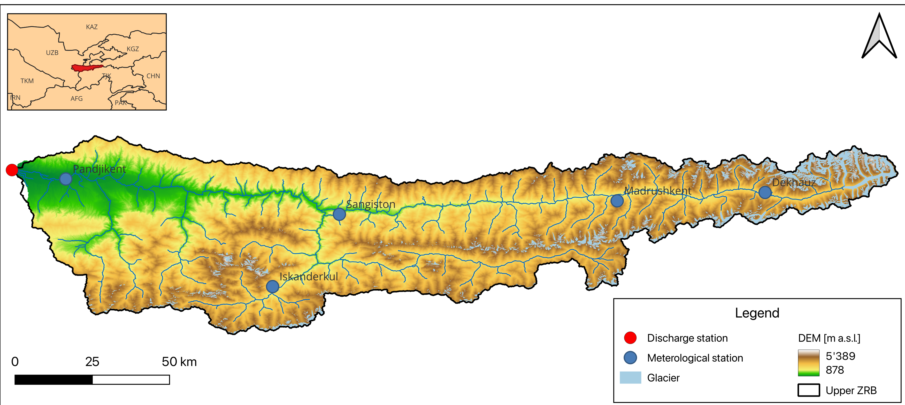
In this exercise, we will also learn how to create a map visualizing your study area and a map illustrating the different land cover types, similar to the one shown in Figure 12.6 and Figure 12.7 for the upper ZRB.
This will be done in several parts, each supported by tutorial videos in both English and Russian:
Part 1: DEM Land Cover
Part 2: Glacier outlines and Study area map
Part 3: HRU’s
Part 4: Discharge data
Part 5: Climate data
Part 1: DEM and Land Cover
In this chapter, we will fill out the sections Geography and Land Cover in Table 1 and download the digital elevation model and land cover data within our catchment boundaries, which we delineated in ?sec-watershed-delineation. To download the DEM and Land cover data we will use the Google Earth Engine (GEE). Google Earth Engine is a cloud-based platform for planetary-scale environmental data analysis. It hosts a vast amounts of environmental data, enabling users to download and perform various analyses and processing tasks.
In this part of the exercise, we will use the GEE to download the SRTM Digital Elevation Model and Land Cover data (Source) and calculate Land cover type statistics using the GEE Link in combination with the following tutorial.
There are several other ways to download the DEM and Land Cover data. Here is a turorial how to donwload the DEM from the Earth Explorer or use the QGIS Plugin. Land cover data can also be obtained directly from the ESA WorldCover webpage.
English version:
Russian version:
Part 2: Glacier outlines and visualization
In the second part of this exercise, we’ll download glacier outlines from the Randolph Glacier Inventory (RGI) v7.0. For more details, refer to #sec-glacier-outlines. The tutorial videos in English and Russian explain how to download the data and import it into QGIS. They also demonstrate how to visualize the data and how to produce the study are map in Figure 12.6 and the Land cover map in Figure 12.7.
English version:
Russian version:
Part 3: Discharge data
Part 4: Climate data
12.3 Conceptual Model Setup
Exercise 3: Chirchik River Basin Conceptual Model Setup
12.4 Delineation of Hydrological Response Units
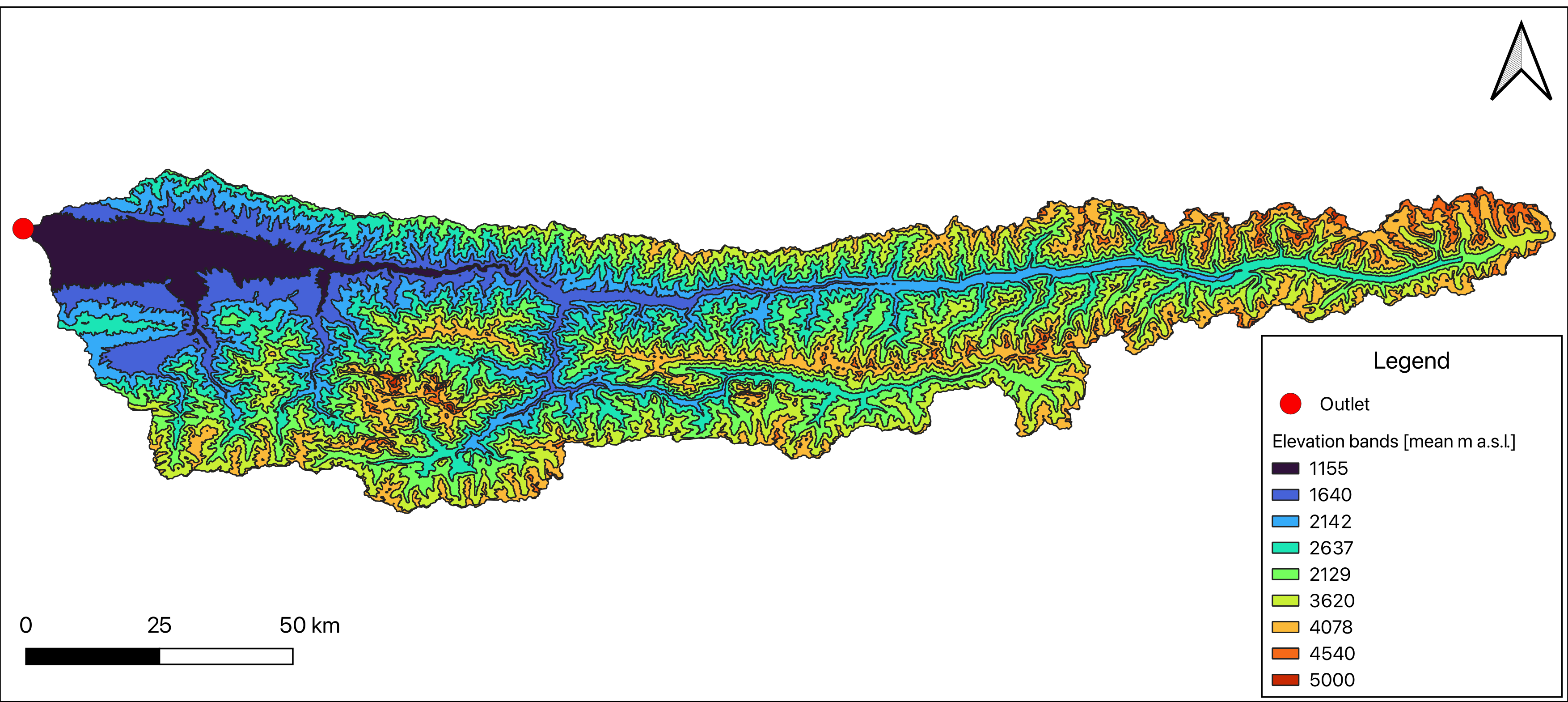
Hydrological response units (HRUs) are areas that have common properties which are important from the hydrological perspective for runoff generation: for instance, similar slope, elevation, aspect, soil type, vegetation cover, landuse. They are areas of land that are assumed to respond similarly to weather input. In each HRU the land-based portion of the hydrological cycle is simulated. HRUs are used in hydrological models to represent the spatial variability of the catchment. The number of HRUs in a catchment depends on the spatial variability of the catchment and the resolution of the input data.
Exercise 4: Hydrological response units (HRUs)
In the fourth part of the exercise, we will utilize elevation bands to delineate HRUs, as elevation significantly influences hydrological processes like precipitation patterns and temperature gradients. Refer to Figure [insert figure number] for an illustration of elevation bands in the upper Zarafshan River basin, as an example for this approach.
12.5 Preparation of Climate Forcing Data
Introductory words.
12.5.1 Historical Climate Data (CHELSA V21 Data)
12.5.2 GCM Simulation Data
12.5.3 Bias-Correction of GCM Climate Data
12.6 Implementation of Hydrological Model
12.6.1 Baseline Hydrological Model
12.6.2 Computing Climate Change Scenarios
12.7 Discussion and Conclusion
12.8 References
Heberger, Matthew. 2022. “Delineator.py: Fast, Accurate Global Watershed Delineation Using Hybrid Vector- and Raster-Based Methods.” Zenodo. https://doi.org/10.5281/zenodo.7314287.
“NASA Shuttle Radar Topography Mission (SRTM).” 2013. NASA. https://earthdata.nasa.gov/learn/articles/nasa-shuttle-radar-topography-mission-srtm-version-3-0-global-1-arc-second-data-released-over-asia-and-australia.
RGI Consortium. 2023. “Randolph Glacier Inventory - a Dataset of Global Glacier Outlines, Version 7.” National Snow; Ice Data Center. https://doi.org/10.5067/F6JMOVY5NAVZ.
Zanaga, Daniele, Ruben Van De Kerchove, Wanda De Keersmaecker, Niels Souverijns, Carsten Brockmann, Ralf Quast, Jan Wevers, et al. 2021. “ESA WorldCover 10 m 2020 V100.” Zenodo. https://doi.org/10.5281/zenodo.5571936.