Appendix C — Quick Guides
Earth Explorer: Register for an Account
In your internet browser, navigate to https://earthexplorer.usgs.gov/. The window will look similar as in Figure C.1.
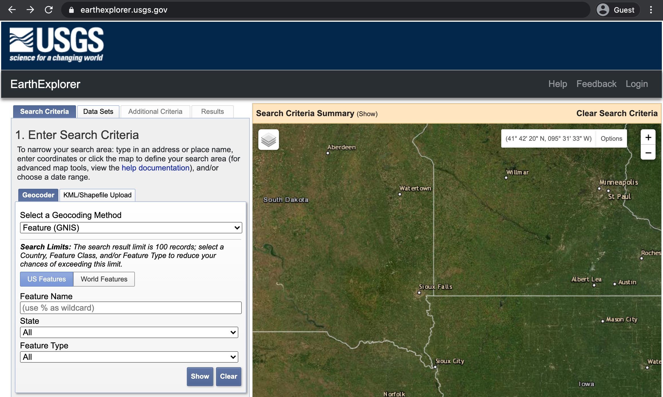
Click on Login in the top right corner. This will bring you to a new window where you can click on Create New Account which will open a form where you enter your information. After verifying your account by clicking on the appropriate link that you will be sent, you can download data from the Earth Explorer interface.
EE: Download SRTM Data for a Selected Region
- Login to the Earth Explorer (Register if you haven’t done so before How to).
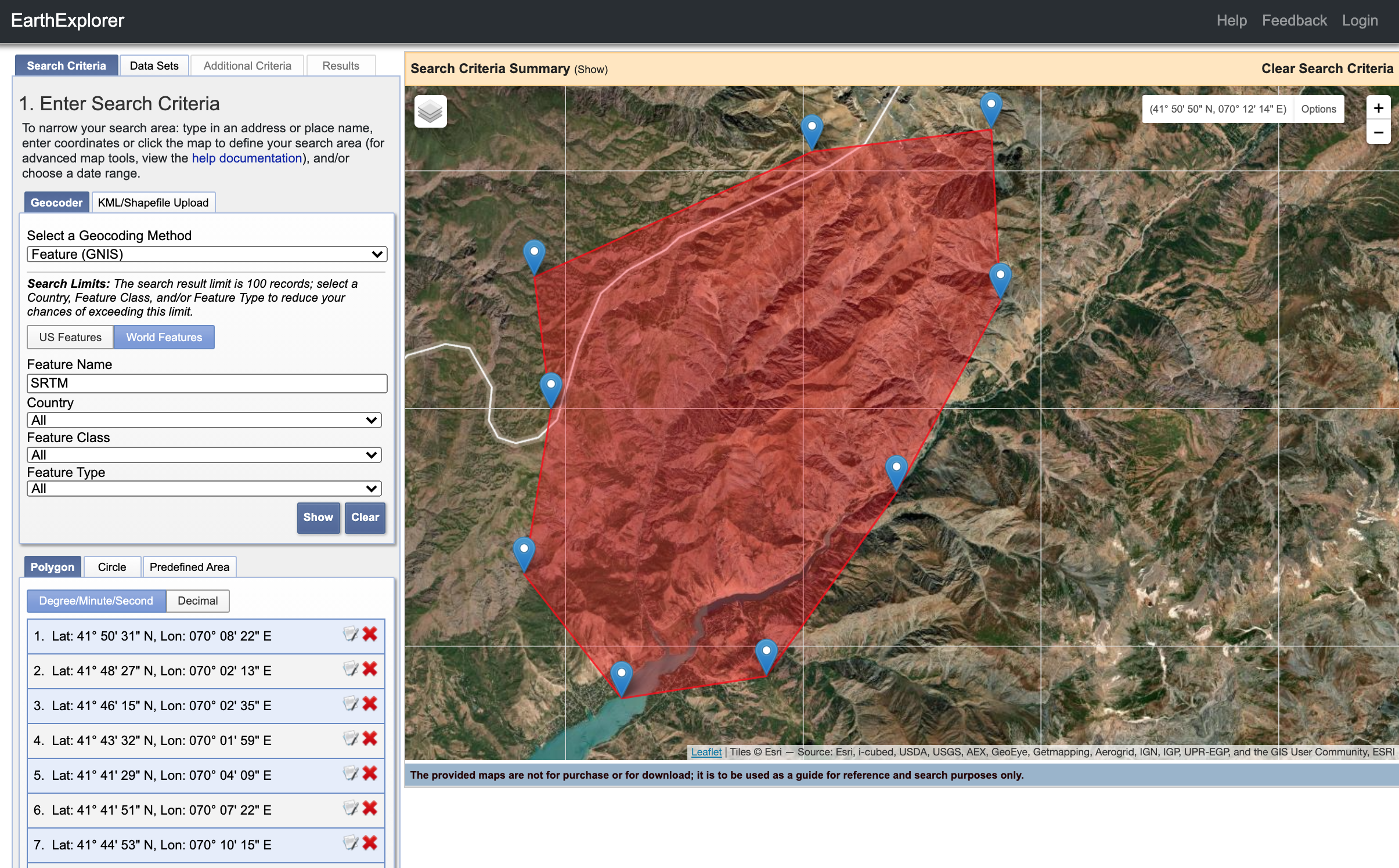
- Navigate to your area of interest in the map panel of the Earth Explorer interface.
- Draw a polygon around your area of interest by clicking on the map (see Figure C.2).
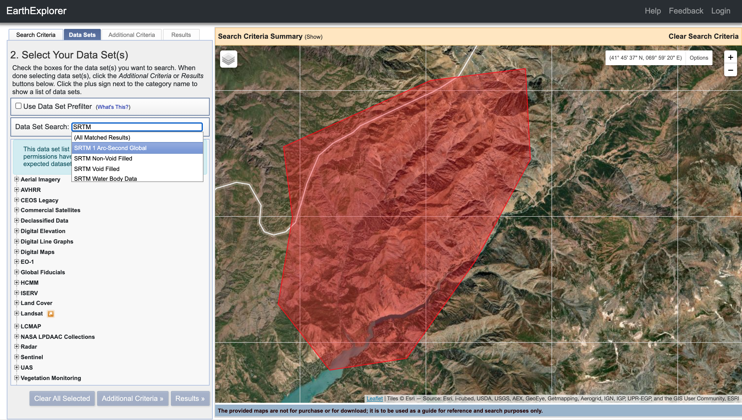
- In the Data Set tab, look for the SRTM 1 arc-second global DEM (see Figure C.3) and select it by ticking the box next to the product name in the list.
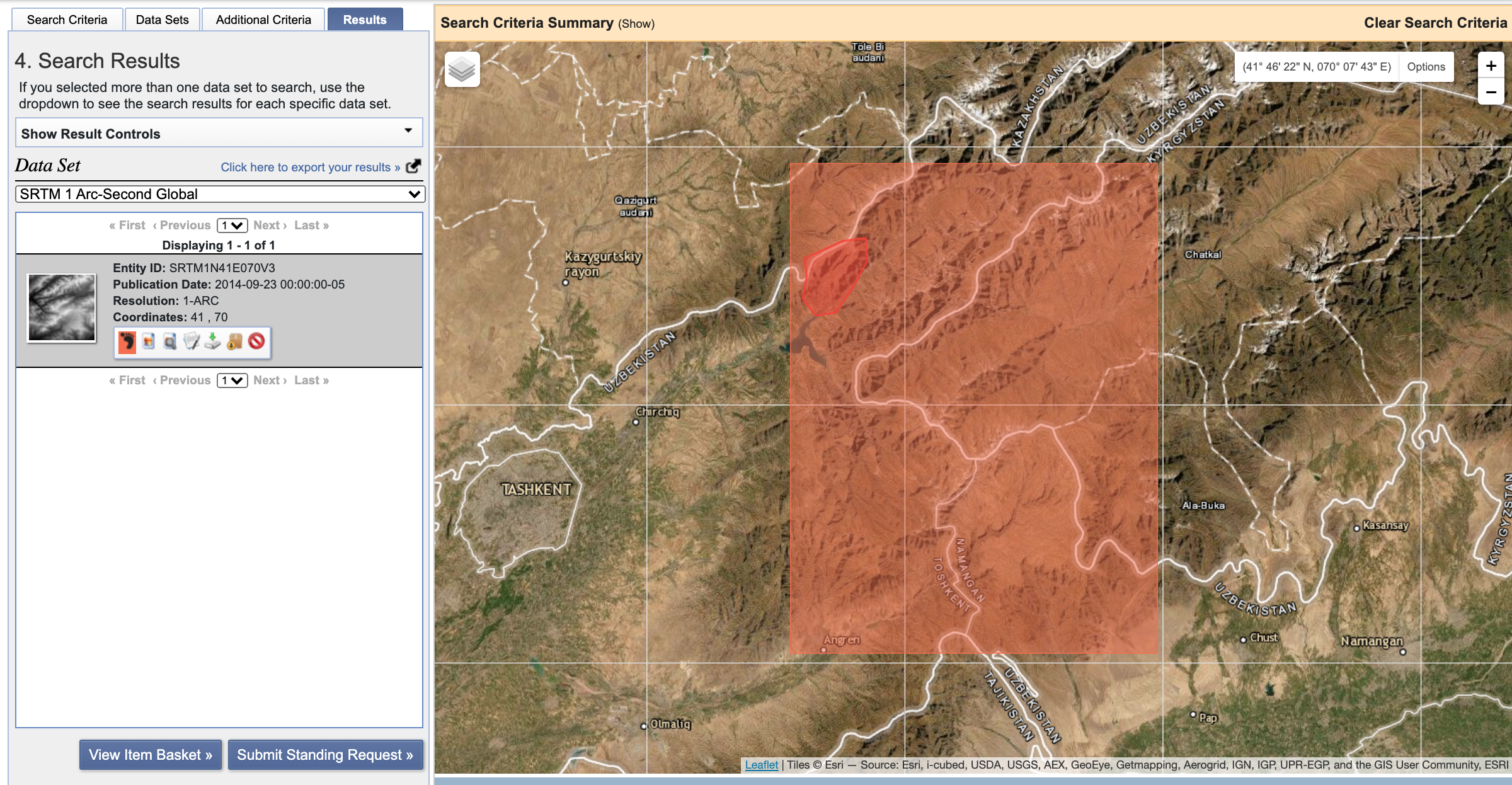
- Verify that the result layer(s) cover your area of interest by pressing the foot icon in the Results tab and download if you are satisfied (Figure C.4).
Back to the Load DEM section.
QGIS Installation Guide
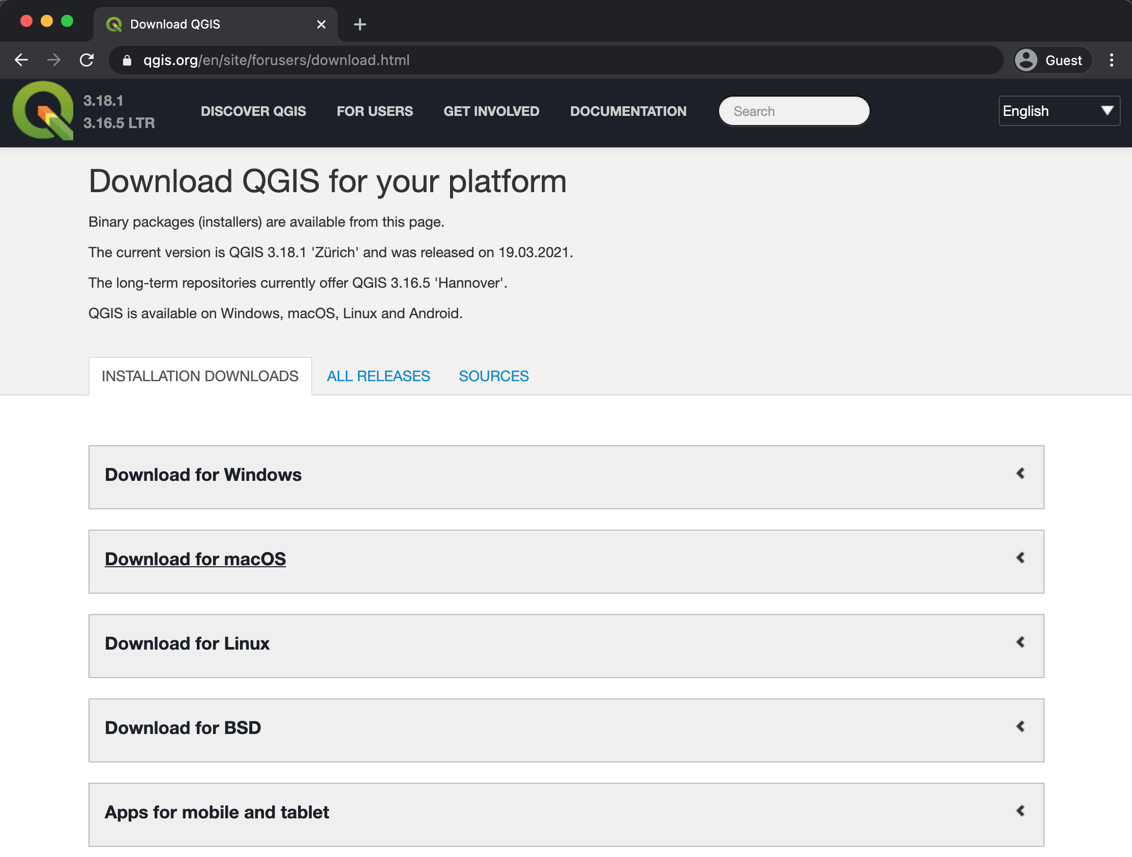
In your web browser go to https://qgis.org/en/site/forusers/download.html (see Figure C.5).
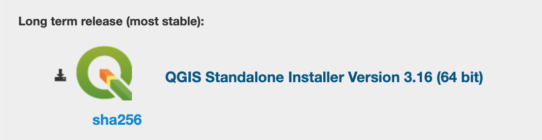
Choose the long-term support version of QGIS for your operating system (e.g. if you use a laptop with a 64-bit Windows operating system, open the Download for Windows tab and click on QGIS Standalone Installer Version 3.16 (64 bit), see Figure C.6)). Clicking on the installer will start the download.
Double-click on the downloaded file to start the installation. Typically, SAGA GIS and GRASS GIS are installed alongside QGIS if you choose this installing option.
The QGIS Window - Overview
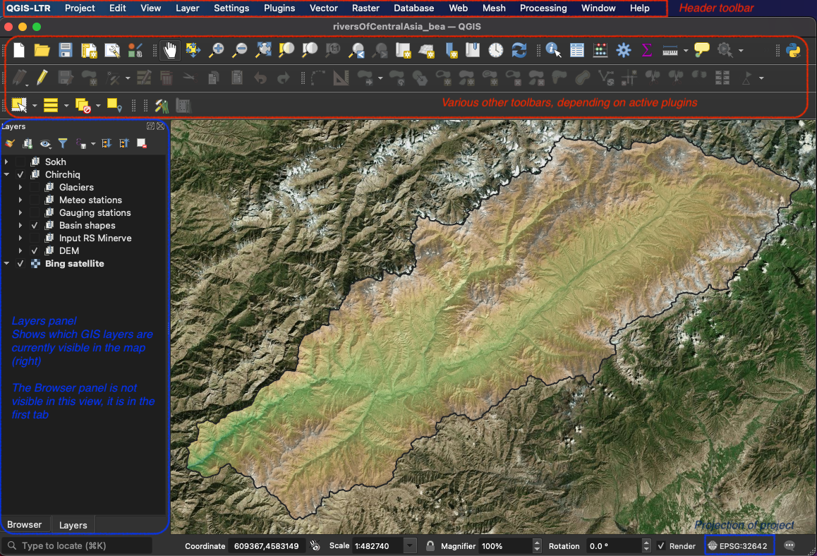
The main parts of the QGIS window which are referenced in this tutorial, are highlighted in Figure C.7.
QGIS: Saving a New QGIS Project
Open your QGIS and open a new QGIS project by moving your cursor on the white sheet symbol in the upper-left corner of your QGIS window (see Figure C.8).
Save the QGIS project by pressing on the disk icon and selecting a location for the file on your computer and a name for the project. You can add freely available on-line maps as background.
Back to setting up of QGIS.
QGIS: Change the Projection of the QGIS Project
For this tutorial, the projection of the QGIS project should be in EPSG:32642 (i.e., UTM 42 N). Change it by clicking on the projects projection in the lower right corner of the QGIS window (see Figure C.7). In the coordinate reference system (CRS) tab of the Project Properties, select WGS84 / UTM zone 42N with ID EPSG:32642 and click OK.
For modeling your own sample catchment, a different UTM zone may be applicable. The map in the lower right corner of the Project Properties window shows the area for the projection in red and the area where your data is located in violet so you can visually verify that you choose an appropriate projection.
Generally, you want to choose the CRS so that you have minimal distortion through the projection in your area of interest. The CRS with ID EPSG:32462 suits well for all of the student exercise catchments.
Back to the setting up of QGIS.
QGIS: Install and activate plugins in QGIS3
Navigate to Plugins in the header toolbar and go to Manage and Install Plugins …. Search for the plugin name and go to Install Plugin to install a plugin or tick the box to the left of the plugin name in the list of plugins to activate it (see Figure C.9).
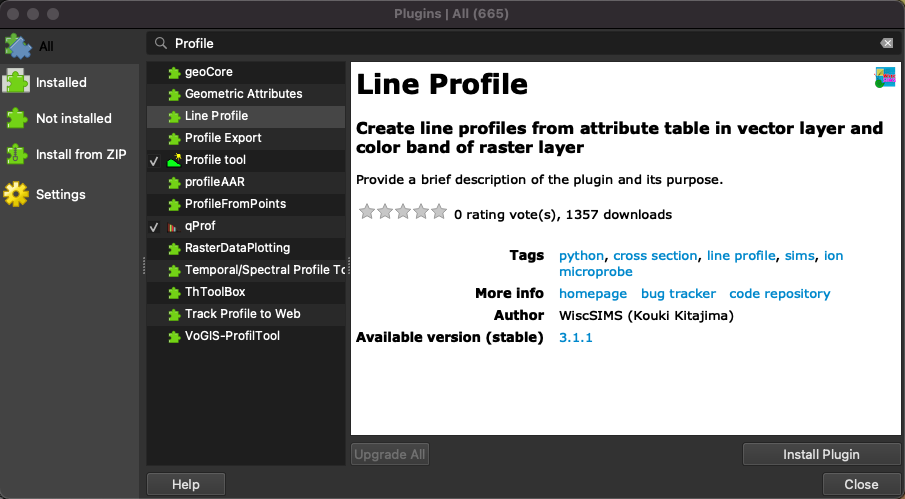
Install Plugin button. Activate installed plugins by ticking the box in the list.
Back to the setting up of QGIS.
GQIS: Managing Panels Visibility in QGIS
Should one of the panels described here not be visible in your QGIS window navigate to View in your header toolbar and then to Panels. The visible panels are marked with a tick. Click on a panel name in the list to activate or deactivate it.
Back to setting up of QGIS.
QGIS: Loading Public Background Maps
You can add freely available on-line maps as backgrounds. Note that they will only be available as long as your computer is connected to the internet. In the Browser panel (see What to do if you don’t see the Browser panel), move the cursor to XYZ Tiles, do a right-click and select New Connection. Enter a descriptive name for the map layer and one of the links below and click OK. The new map layer will appear under XYZ Tiles. By double-clicking on the layer you can add it to your Layers panel.
Back to setting up of QGIS.
QGIS: Zoom to Layer
You can tell QGIS to zoom to the selected layer by selecting a layer in the Layers window and then on the white sheet and magnifying glass icon in the toolbar (see Figure C.10).
You can also perform a right-click on the layer name in the Layers panel and select Zoom to layer.
QGIS: Import SRTM layers using the SRTM plugin
Make sure the SRTM plugin is installed (see How to). Navigate to Plugins in the header toolbar and there to SRTM Downloader. Select the SRTM Downloader. Set the boundaries of the SRTM tiles to download and press the Download button. Close the window when done. The SRTM tiles are loaded to the Layers pane.
Back to Load DEM in QGIS section
QGIS: Merge SRTM Tiles to a Single Layer
Navigate to Raster in the header toolbar and then to Miscellaneous and Merge…. In the Merge window that opens, select the input layers by clicking on the … button. Tick the layers that need to be merged and press Run. When the algorithm is done, close the window. You can zoom to the extent of the new layer (see How to). You can change the color of the DEM file.
Back to Load DEM in QGIS section
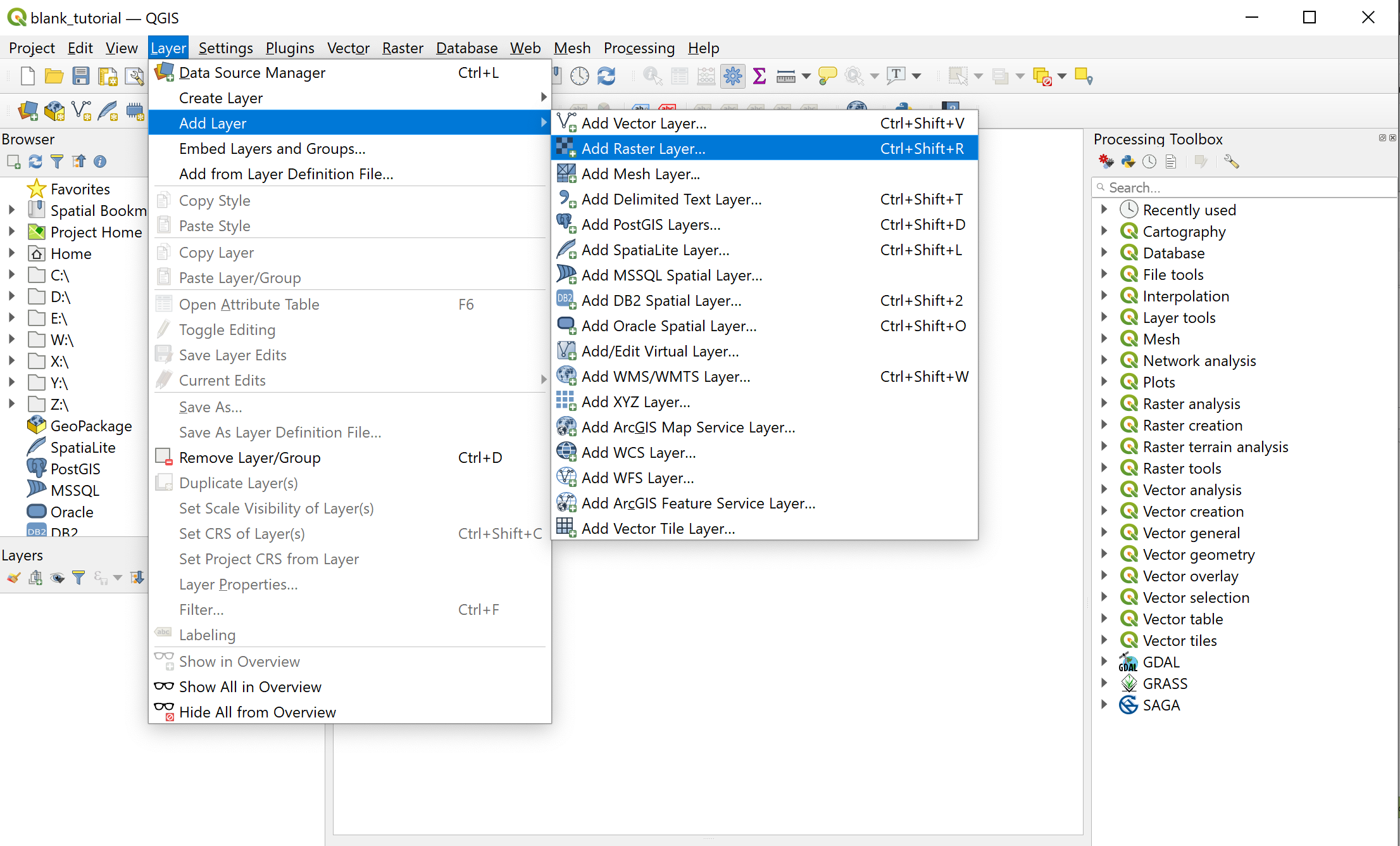
QGIS: Add Raster Layer
In your QGIS window, navigate to Layer in your header toolbar, there to Add Layer and left-click on Add Raster Layer (see Figure C.11). The Data Source Manager will open in a pop-up window (see Figure C.12).
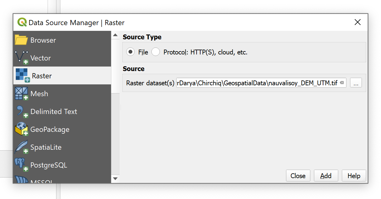
In the example above, a DEM for the example of the Nauvalisoy river catchment is loaded. For loading the DEM of your sample catchments, browse for the DEM in the corresponding folder you downloaded from the provided Dropbox directory.
Press the Add button at the bottom right of the Data Source Manager window to load the raster layer to your QGIS project and close the window by pressing the Close button (to the left of the Add button).
Your QGIS project now shows a grey-scale version of the raster layer you loaded. If you are satisfied with the change, save your project by pressing the disk icon at the upper left corner of your QGIS window.
You can change the color of your raster file (how to). Here is a quick-guide of how to apply a topography-style color band to your DEM.
QGIS: Change Color of Raster Layer
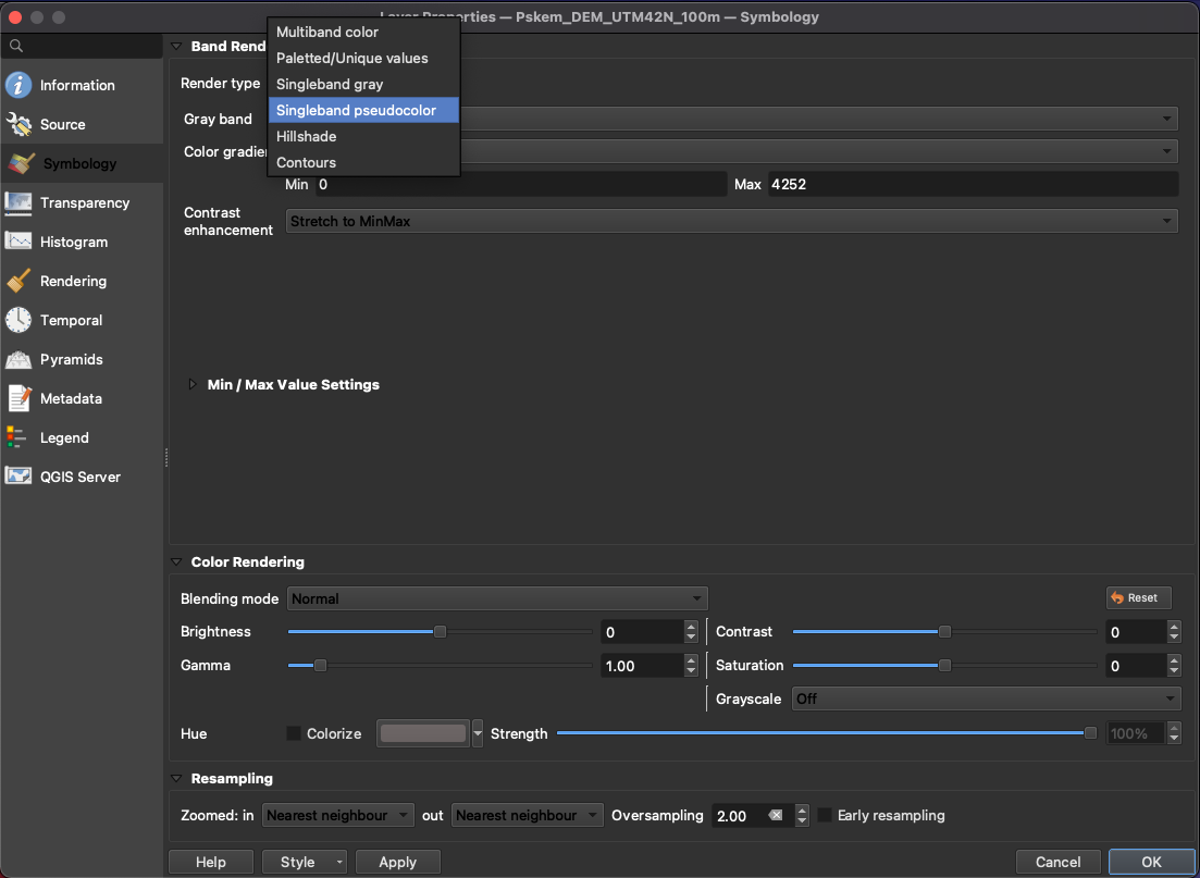
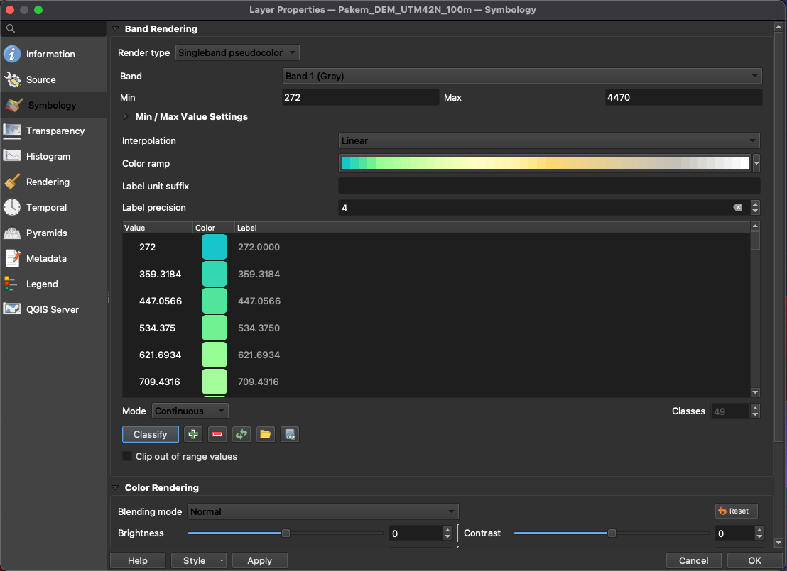
You can change the colors of your cut DEM by double-clicking on the layer name in the Layers window. Go to tab Symbology (with the paint and brush icon) and choose Render type Singleband-pseudocolor (see Figure C.13) and select a Color ramp.
QGIS comes with a large library of color ramps but you can also create your own. See below a description of how to get your DEM in a topography style color palette.
QGIS: Topography-style color palettes
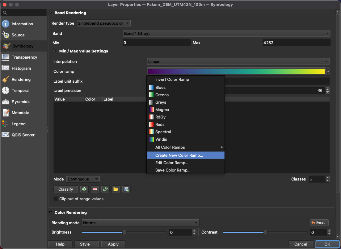
For our DEM we choose an existing topography-style color ramp. Open the Layer Properties window with a double-click on the raster layer in the Layers pane of the QGIS window. In the Symbology tab click the triangle to the right of the color ramp and select Create New Color Ramp… (see Figure C.14).
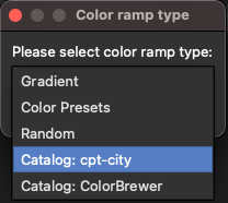
In the drop down menu of the pop-up window choose Catalog: cpt-city and press OK (see Figure C.15).
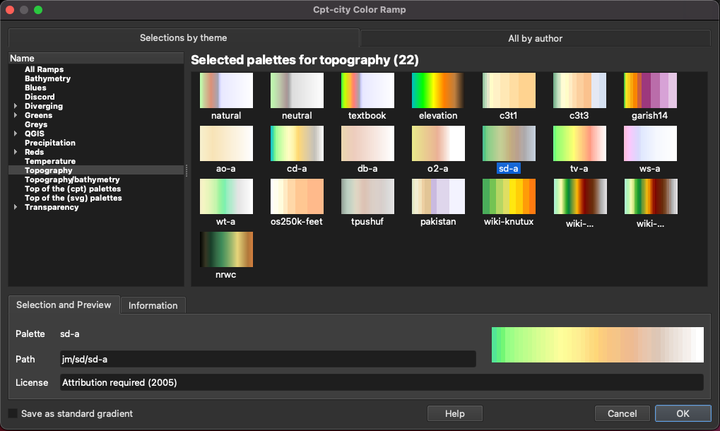
A this will open another window containing the catalog of existing color ramps. Under Topography, we choose sd-a and press OK (see Figure C.16).
Go to tab Transparency, set Global Opacity to 30% and specify the No Data Value 0 (see Figure C.17).
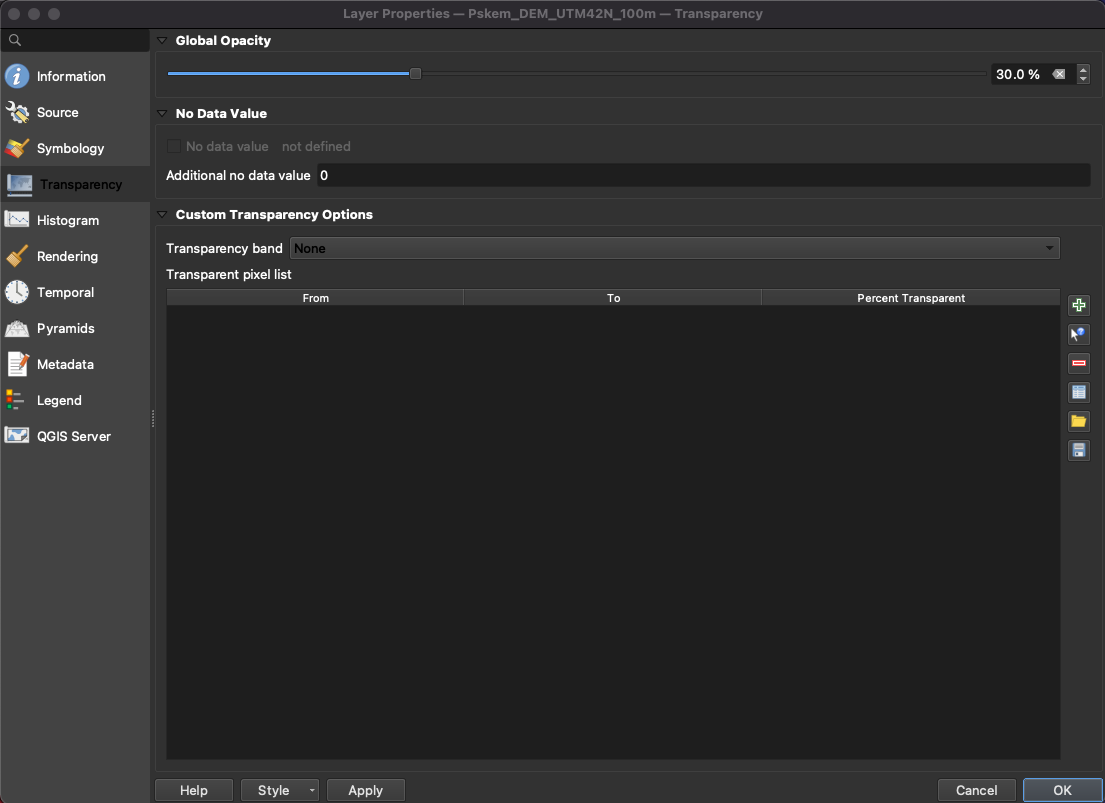
Then go back to the Symbology tab. The minimum value of the color ramp should now not be 0 but 272. Adapt manually if need be. Then, press classify to get a discrete color ramp for your map and Apply to the map. If you are happy with the colors, quit by pressing OK (see Figure C.18).
The result will look like Figure C.19.
You can add decorations (e.g. scale and north arrow) to your map (how to).
QGIS: Add Map Decorations
Navigate to View -> Decorations and choose among the decorations to add. Many options for configuring the decorations are available.
C.1 QGIS: Verify Projection of Layer and Re-project Layer
Open the Layer Properties window with a double-click on the layer in the Layers pane and navigate to the Information tab. Under CRS (coordinate reference system) you see the projection of the layer. For the Chirchiq river basin, the CRS should say “EPSG:32642 - WGS 84 / UTM zone 42N - Projected”. Other river catchments in Central Asia may require a different UTM zone. For the student exercises, it is good to choose this projection for all basins.
A raster layer can be reprojected to a different CRS: Go to Raster in the header toolbar. From there move the cursor over Projections and click on Warp (Reproject)…. The Warp window will pop up (in fact, it is just an interface where the user can specify the parameters of the wrap algorithm in a convient way). Select the raster layer you wish to re-project in the Input layer and select the Target CRS.
If the target CRS you wish to re-project to is not available in the drop-down menu, you can browse for it by clicking on the globe icon to thr right of the Target CRS section. You may re-sample the raster to a coarser resolution by specifying the Output file resolution. You may also specify to save the reprojected raster layer: Scroll to the bottom of the Warp (Reproject) window where you see Reprojected and a white box where you can browse for a location to store the new layer.
If you do not specify a target location, only a temporary layer will be loaded to QGIS which will not be available anymore after you close the QGIS project (even if you save the project).
You may decide to load the temporary file and save it later (how to). Click the Run button at the bottom right to start the re-projection algorithm and press Close when the process is done. The reprojected layer will be available in the Layers pane.
A vector layer can be reprojected by selecting Vector in the header toolbar, moving the cursor to Data Management Tools and clicking on Reproject Layer…. This opens the Reproject Layer window where you can specify a Target CRS and optionally a storage location. As for the reprojection of the raster layer, a temporary layer is loaded to your QGIS project if you do not specify a storage location. However, you can always store temporary layers later (how to).
Back to the load DEM section.
QGIS: Save a Temporary Layer
Right-click on a temporary layer in the Layers pane. Temporary layers are indicated by a box to the right of the layer name. From the menu that opens upon right-click, select Export and Save As… (for raster layers) or Save Feature As… (for vector layers). An explorer window will open where you can specify a file name and a location to store the file to.
QGIS: Add Vector Layer
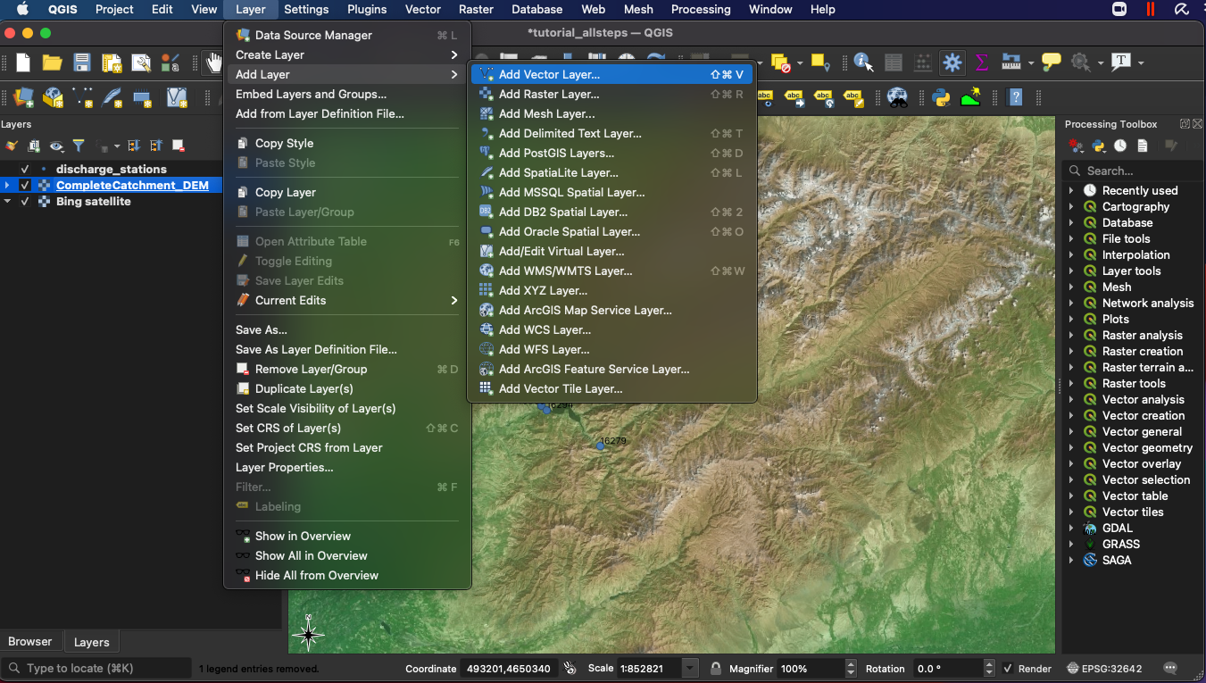
Left-clicking on Layer, moving your cursor over Add Layer and left-clicking Add Vector Layer (see Figure C.20).
A window will pop up, asking you to specify the properties of the vector layer to add (see Figure C.21).
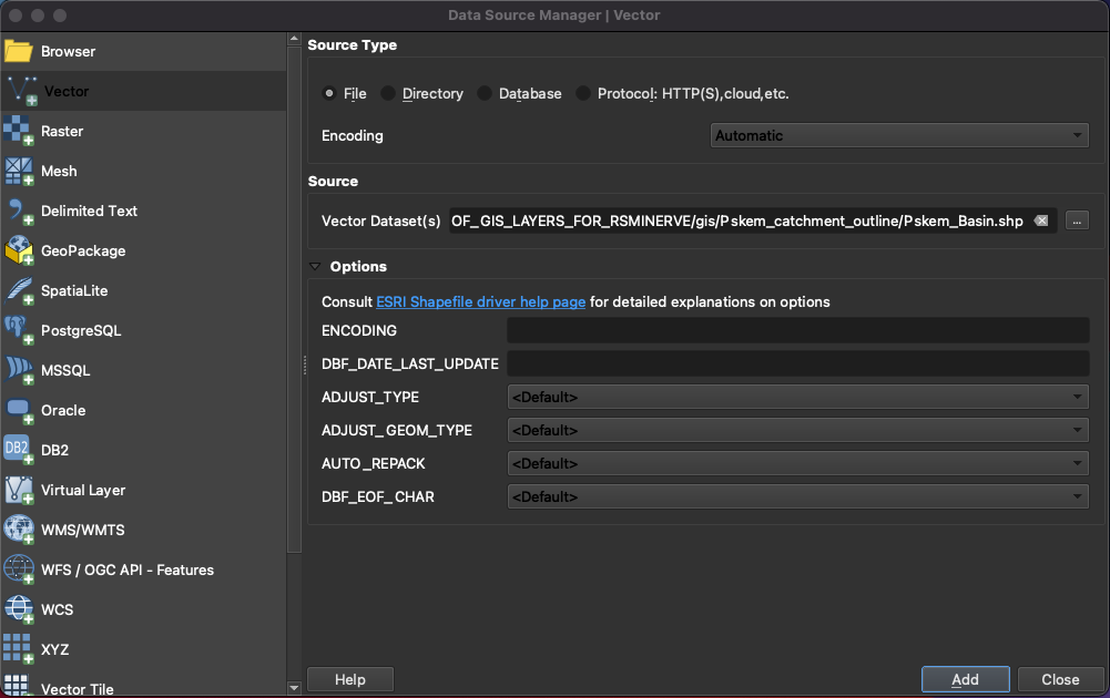
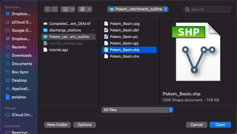
Press the box with the three dots on the right of the source field to specify the location of the shape file to be added to your project (see Figure C.22). Click Open and the window will close. The address of your shape files should now stand in the source field as in Figure C.21.
Note that you load the .shp file but that all the files in the list in Figure C.21 need to be present. In the Add Vector Layer window, click Add and then close the window. QGIS has attributed a random color to your shape file which can be changed manually How to.
QGIS: Change Color of a Vector Layer
You can change the color of your layer by double-clicking on the layer name in the Layers Window to the left of the map. This will open the properties window. The third tab from the top shows paint and brush (see Figure C.23).
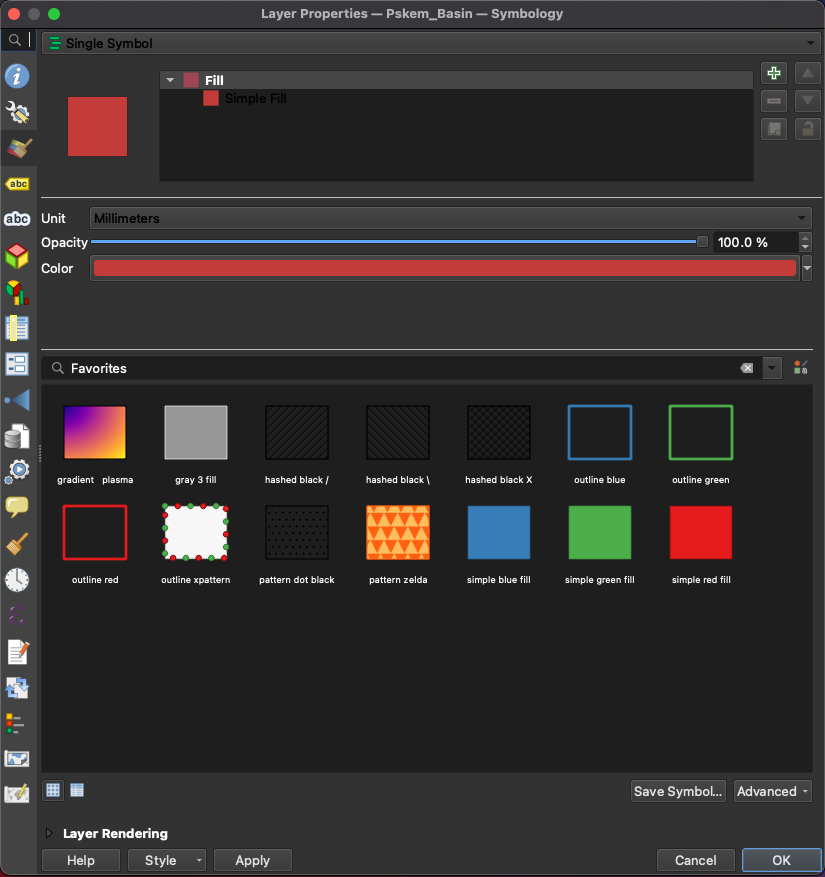
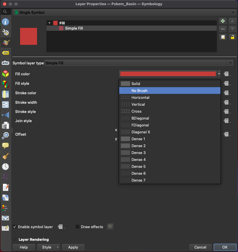
You can activate Simple fill by clicking on it and select No brush in the drop-down menu in order to only show the outline of your vector layer (see Figure C.24).
QGIS: Fill Sinks
Browse for the Fill sinks algorithm in the Processing Toolbox panel (see Figure C.25). If the Processing Toolbox panel is not visible go to Processing in the header toolbar and click on Toolbox to activate it. Alternatively, here is how to manage the visibility of panels in QGIS.
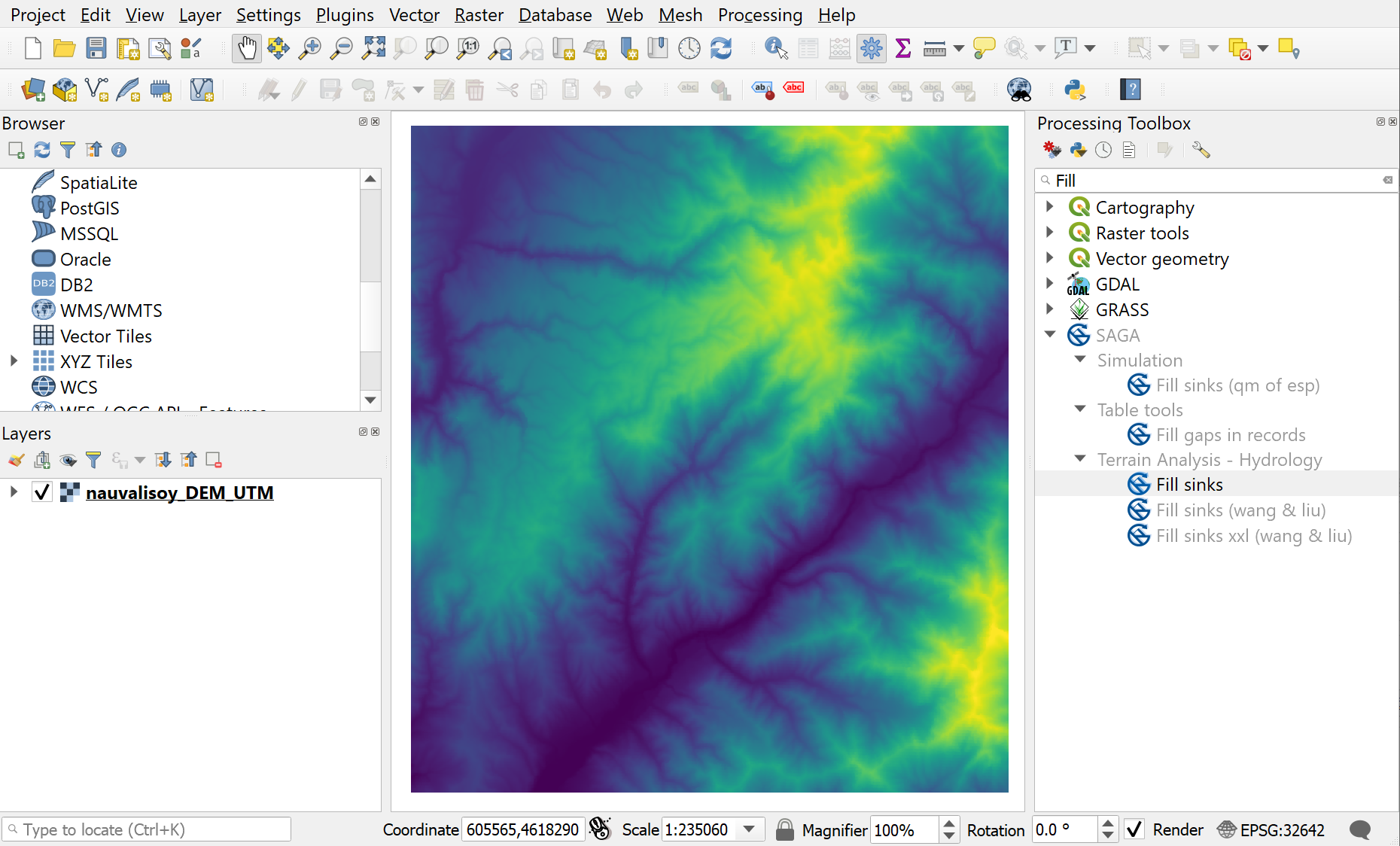
Open the Fill sinks window with a double-click on the name of the algorithm in the Processing Toolbar panel. There, select the DEM you want to process and browse for a location to store the output file (see Figure C.26). You can leave the default minimum slope.
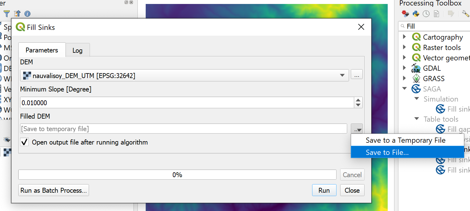
When the algorithm is done it will load the new layer into your QGIS project. Close the Fill sinks window and save your project.
Back to catchment delineation.
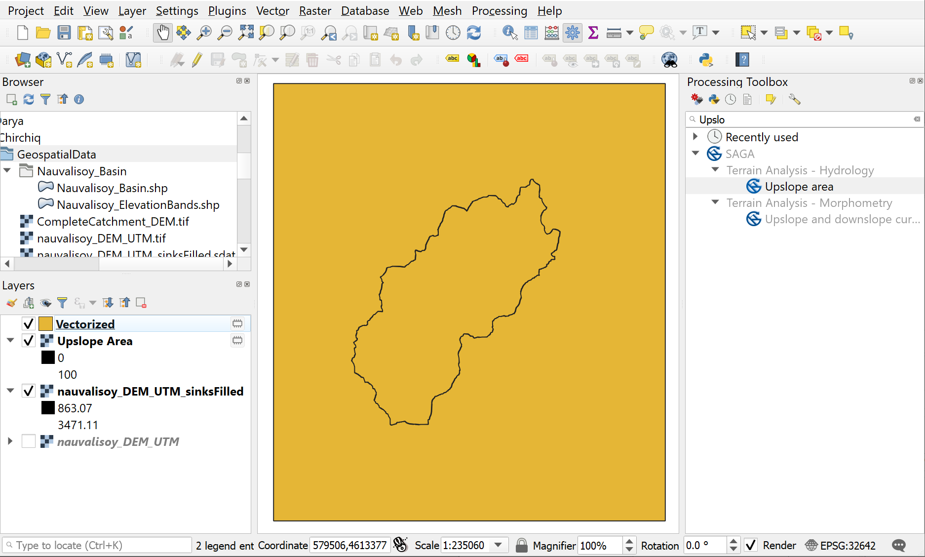
QGIS: Calculate the area upslope of a point
Search for the SAGA algorithm Upslope Area in the Processing Toolbox panel and open the function window with a double click on the name. Enter the Longitude of your discharge station for the Target X coordinate and the Latitude for the Target Y coordinate for which the upslope area should be calculated. For the Elevation select the sink-filled DEM (see how to fill sinks in a DEM and why we need to fill in sinks).
All GIS layers and the coordinates of the discharge gauge need to be in the same UTM projection. Choose a method in the drop-down menue in the Method section and optionally specify a location for the output file. For the example of the Nauvalisoy basin, the Upslope Area window filled in correctly is shown in Figure C.27.
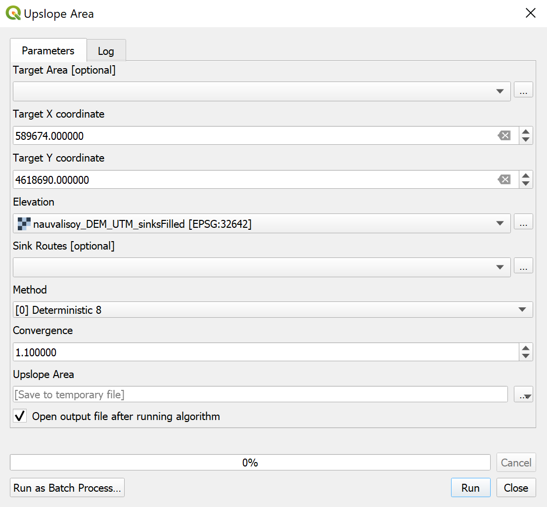
Click Run and Close after the algorithm is done. A new raster file with the values 0 for outside the catchment area and 100 for inside the catchment area is now loaded into your QGIS project.
Back to catchment delineation.
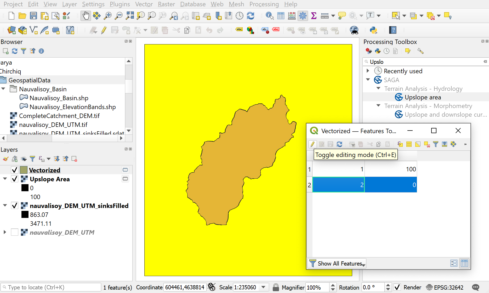
QGIS: Polygonize a Raster
Got to Raster in the header toolbar, move your cursor over Conversion and click on Polygonize (Raster to Vector)… (see Figure C.28).
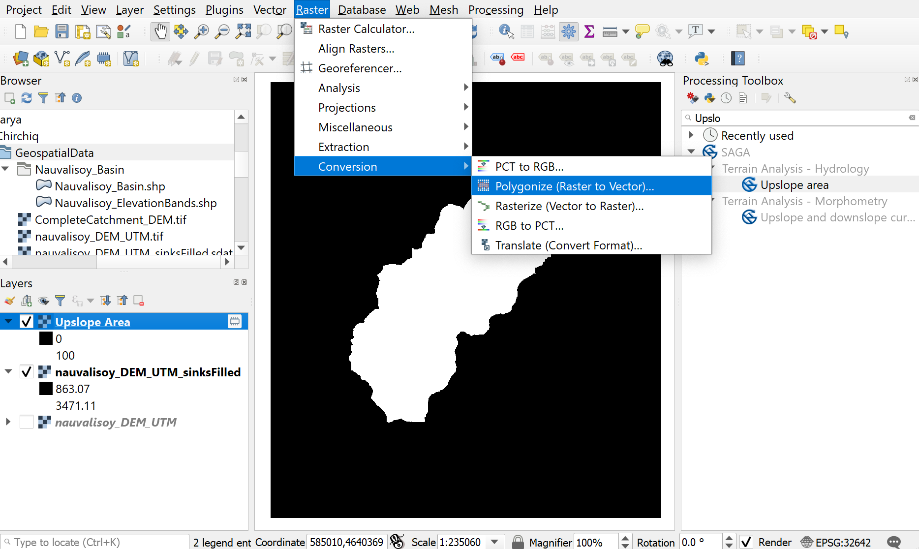
Select the raster layer you wish to polygonize (for example the upslope area raster layer) and run the process. Close the polygonize window after the algorithm is done. A new shape file will be loaded to your GIS project (see Figure C.29).
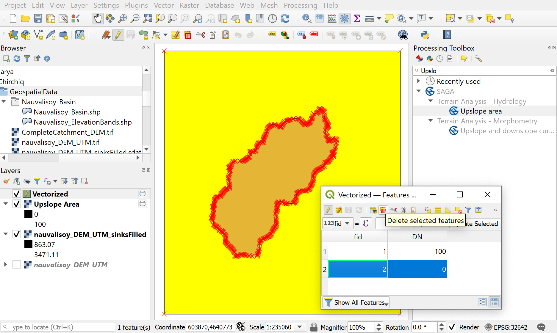
The new vector layer has 2 features: the watershed boundary and a box around the watershed the same size of the DEM we used. To get rid of the outer shape, open the attribute table with a right-click on the vector layer and selecting Open Attribute Table. In the attribute table, elect the outer shape by clicking on the second row of the attribute table and toggle the edit mode by clicking on the pen icon (see Figure C.30).
Delete the outer shape by pressing the red bin icon in the attribute table (see Figure C.31).
Save the edits in the attribute table (see Figure C.32) and press the pen icon again to un-toggle the edit mode.
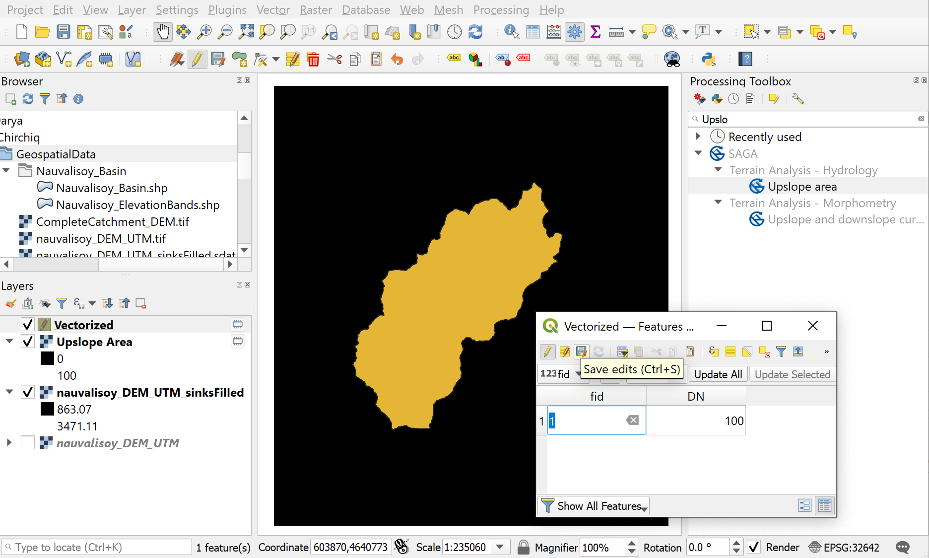
Close the attribute table window and save the boundary of your watershed and your QGIS project.
Back to catchment delineation.
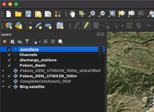
QGIS: Edit Junctions Layer
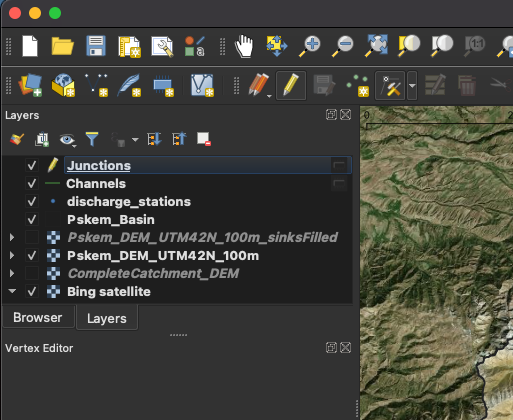
Select the Junctions layer and toggle manual editing by clicking on the yellow pen (see Figure C.33).
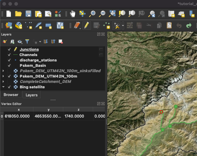
When in editing mode, the yellow pen will appear in the Layers window next to the name of the layer being edited. The edit mode will also activate a button for adding points (i.e. junctions, we don’t need that now) and the vertex tool. Click on the vertex tool icon. It is active when a a boundary appears around the icon and the Vertex Editor windows opens (see Figure C.34).
Right-click on a junction point you would like to delete to activate it (see Figure C.35).
Select the activated point by drawing a rectangle over the point with your mouse. The point will appear blue (see Figure C.36).
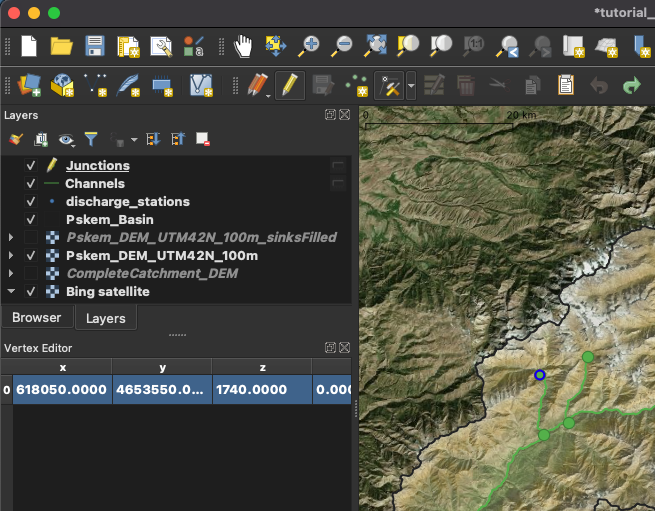
Delete the point with the delete key on your keyboard. You can save your edits by pressing the blue-white Save Layer Edits button that is decorated with an orange pen (see Figure C.37). This saves your changes without exiting the edit mode.
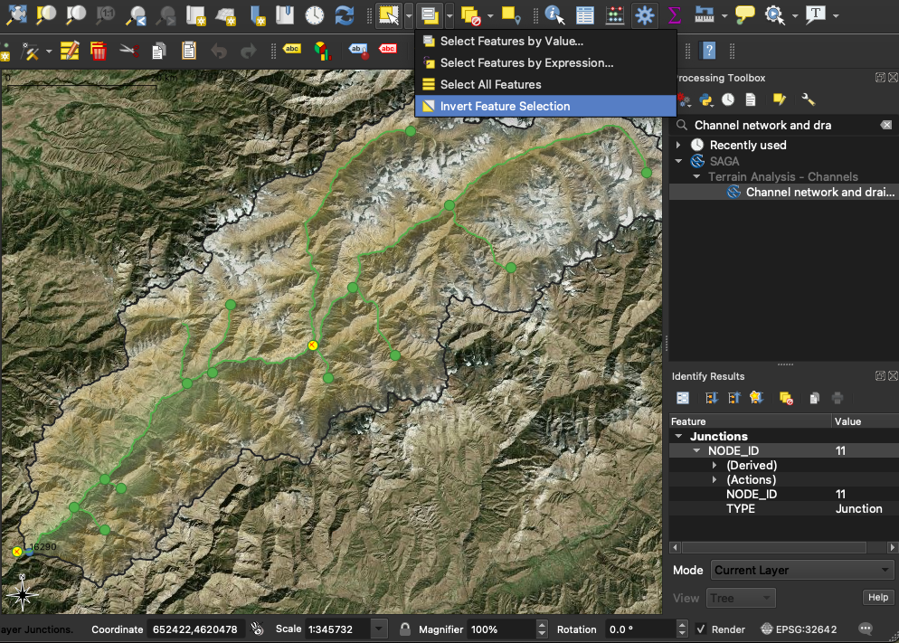
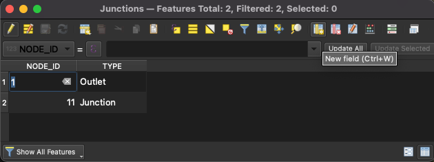
If you have many points to remove, as in our case, it may be faster to identify the IDs of the features you want to keep, select these and delete all others. To start, you activate the Identify Features mode by clicking on the icon with the white i on the blue circle (see Figure C.38).
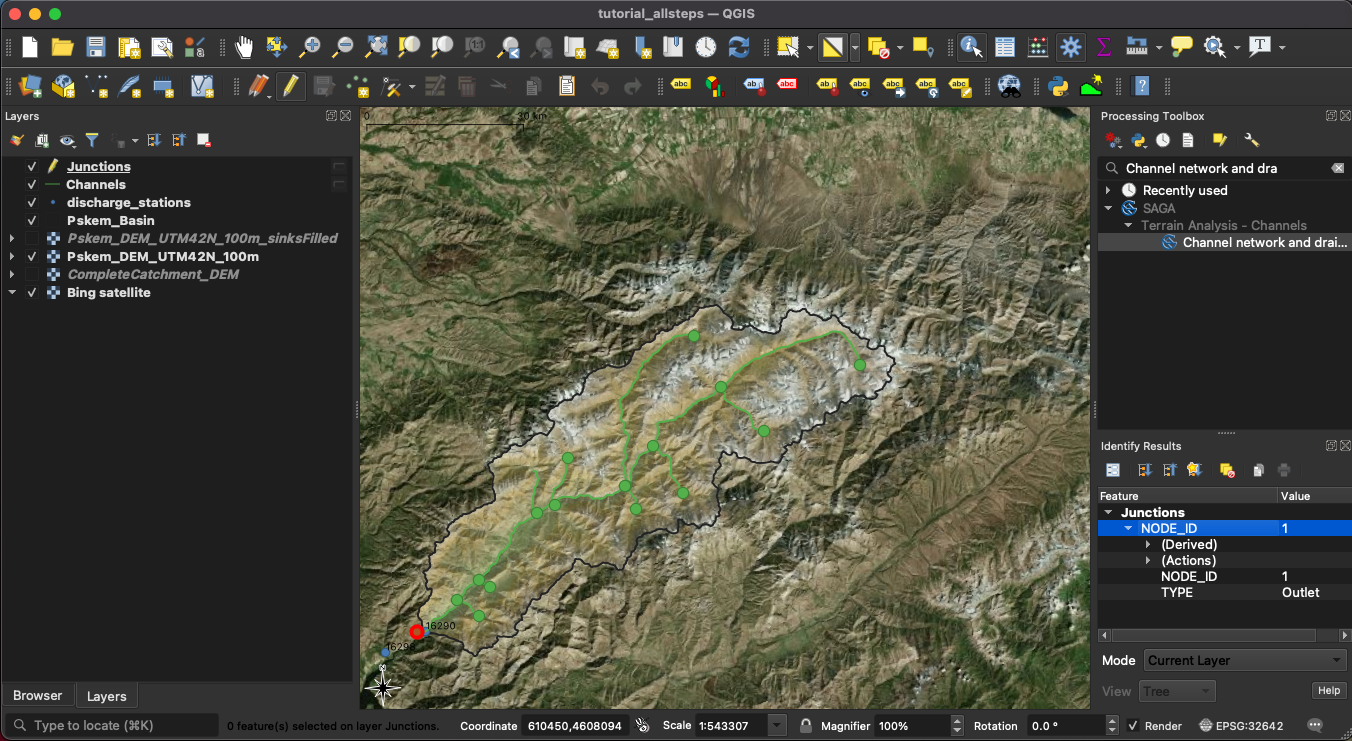
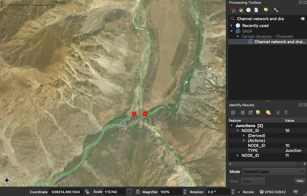
A black i will appear next to your cursor. You then click on the first of your nodes that you want to keep. This will highlight it in red and a list with information on the selected feature appears on the right in the Identify Results window. You will see the attribute NODE_ID with value 1 for the outflow node (see Figure C.39). Note down the ID of the feature.
You then press on the node at the confluence of the two tributaries in the center of the catchment. The Identify Results window shows 2 results, that means, that two junction nodes are close to each other (see Figure C.40).
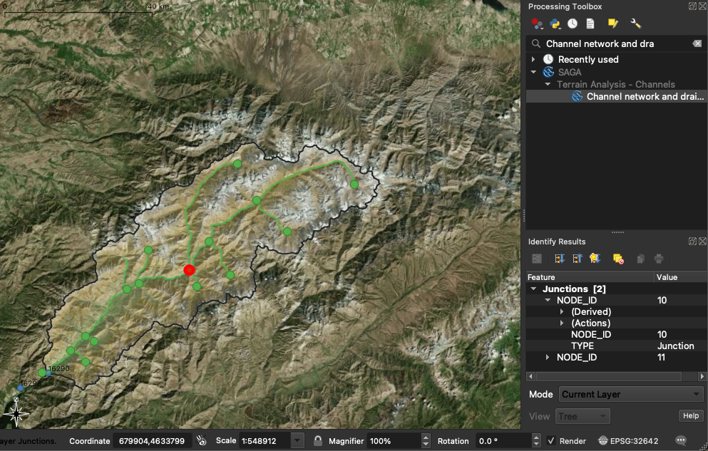
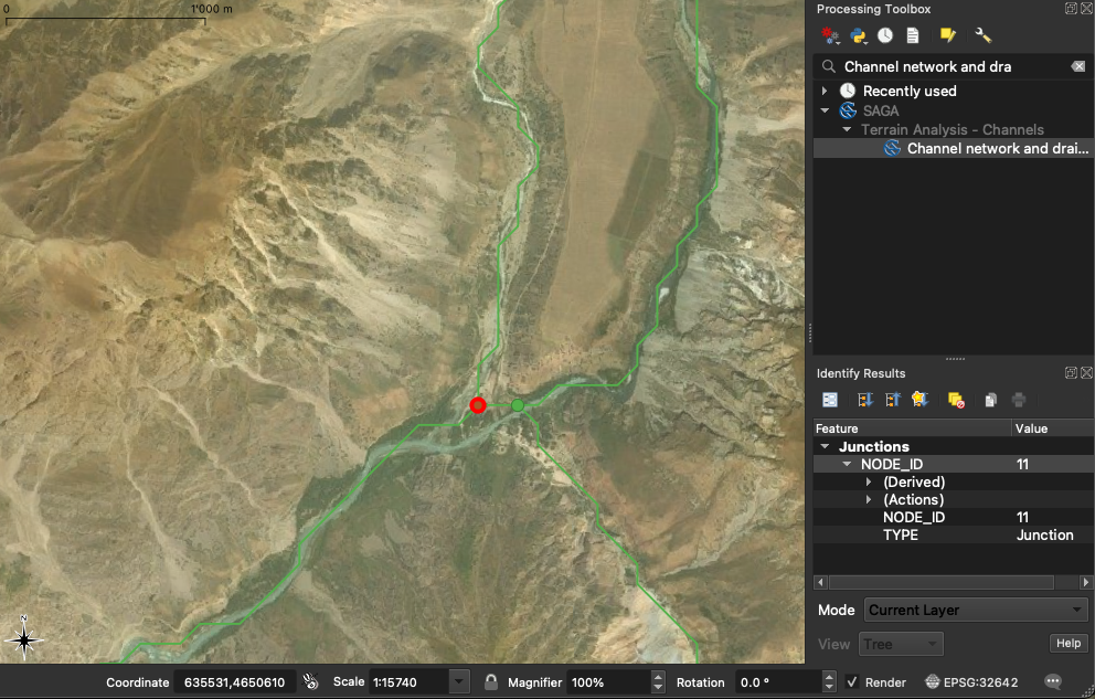
Zoom in in your map window with your mouse to see the two nodes (see Figure C.41).
Select the node that should be kept and not the ID of the node (NODE_ID 11) (see Figure C.42).
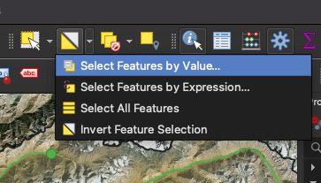
Zoom back to the entire Junctions layer (see Figure C.10) and go to Select Features by Values… in the toolbar (see Figure C.43).
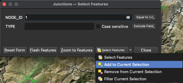
Add NODE_ID 1 to your selection as demonstrated in Figure C.44.
The outflow node with ID 1 will change color in your map as shown in Figure C.45.
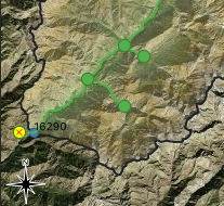
Add node 11 to your selection in the same way and close the Select Node by Value window. Invert the feature selection as shown in Figure C.46.
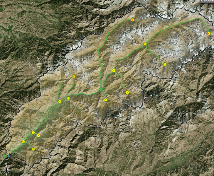
All other nodes will now be yellow and the ones to keep will appear in the layer color (see Figure C.47).
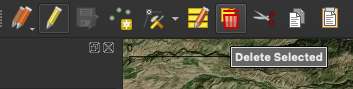
Delete the features (nodes) by pressing the Delete Selected button in the edit features toolbar as shown in Figure C.48.
Save your edits (see Figure C.37). To verify that, indeed, all superfluous nodes are deleted from the Junctions file, open the Attribute table shown in Figure C.49.

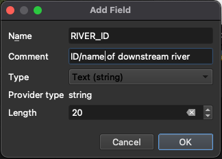
Only 2 features should be listed under each attribute. We will now edit the attribute table to prepare it for the RSMinerve model. RSMinerve needs an identifier to differentiate between the junctions. We can use the attribute TYPE to uniquely identify the two junctions needed. RSMinerve further needs the ID of the downstream river. Add a column to the attribute table by pressing the Add Field button (see Figure C.50).
Define a name for the attribute, a type and admissible length of each entry in the Add Field window. In our case, we choose a string consisting of letters as ID and allow it to be 20 characters long as shown in Figure C.51.
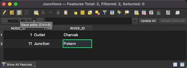
Close the window by pressing OK. By clicking in the newly created NULL fields, you can now type names for the downstream rivers and save your edits by pressing the save edits icon (3rd from the left in the toolbar of the attribute table window). As the outlet of the catchment goes directly into Charvak reservoir, we can type Charvak as the downstream river ID for this example. The river stretch between junction and outlet is called Pskem (see Figure C.52).
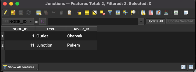
We are done editing the Junctions layer. Deactivate the edit mode by clicking on the yellow pen in the attribute table window as demonstrated in Figure C.53 and close the window.
Now save the Junctions layer in an appropriate place on your drive. Time to save your QGIS project.
In the same way you can also edit the river channels layer.
RSM: Create HBV model and edit parameters
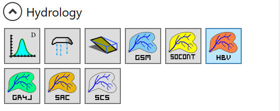
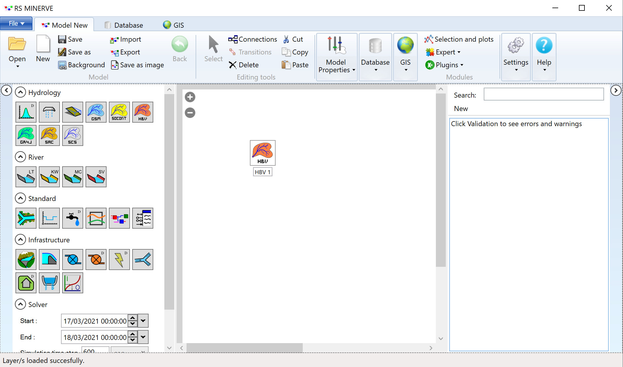
Click on the HBV model icon in the model selection panel (see Figure C.54).
Move your cursor to the white area in the center and create a HBV model with a click. The HBV model icon will now appear in the white model panel (see Figure C.55).
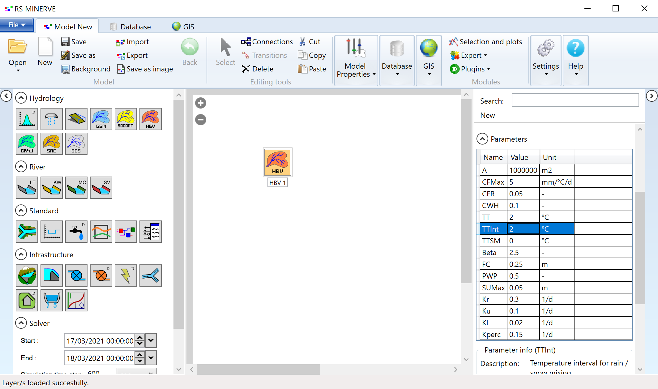
Edit the parameters of the model by double-clicking on the model icon and changing parameter values in the table that appears to the right of the RSMinerve window (see Figure C.56).
Alternatively (especially if you have to change parameters for several models), activate the Parameters panel in the Model Properties toolbar (see Figure C.57).
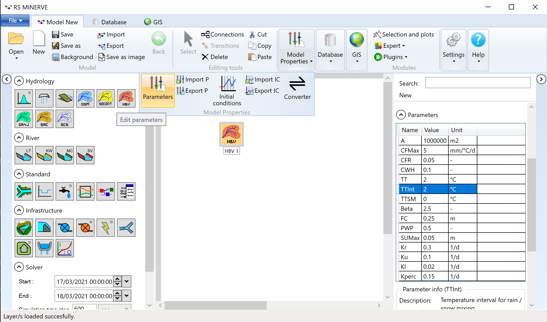
Select the HBV model in the Parameters panel as shown in Figure C.58.
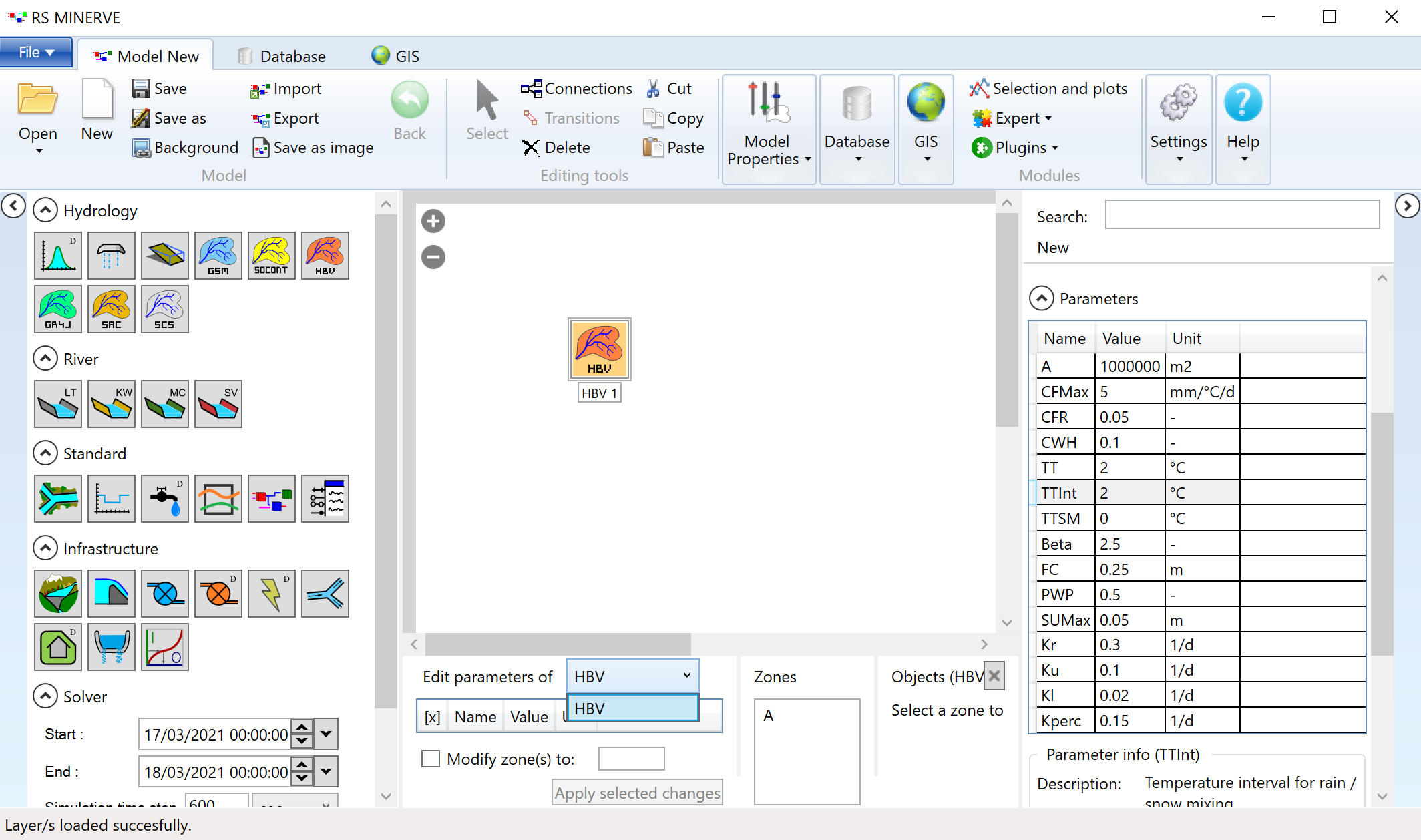
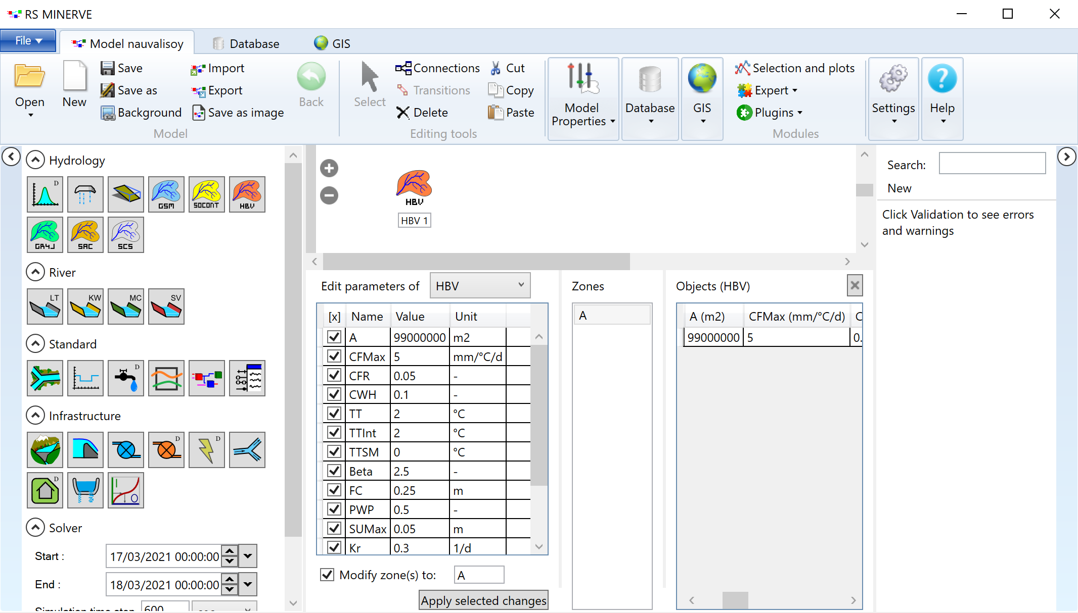
If you have several HBV models, you can select models by zone and apply edits in the parameter table in the left of the Parameters panel to all selected models (marked with tick). You can also edit paramers for individual models in the right-hand table of the Parameters panel as is visible in Figure C.59.
Save your model by clicking the floppy disk icon in the toolbar.
You can also export parameters to a text file via the button Export P in the Model Properties toolbar, edit the text file and import the edited parameter file through Import P.
Note that for the Nauvalisoy demonstration case study, the area of the HBV model should be 99’000’000 m2.
Back to the Nauvalisoy model guide.
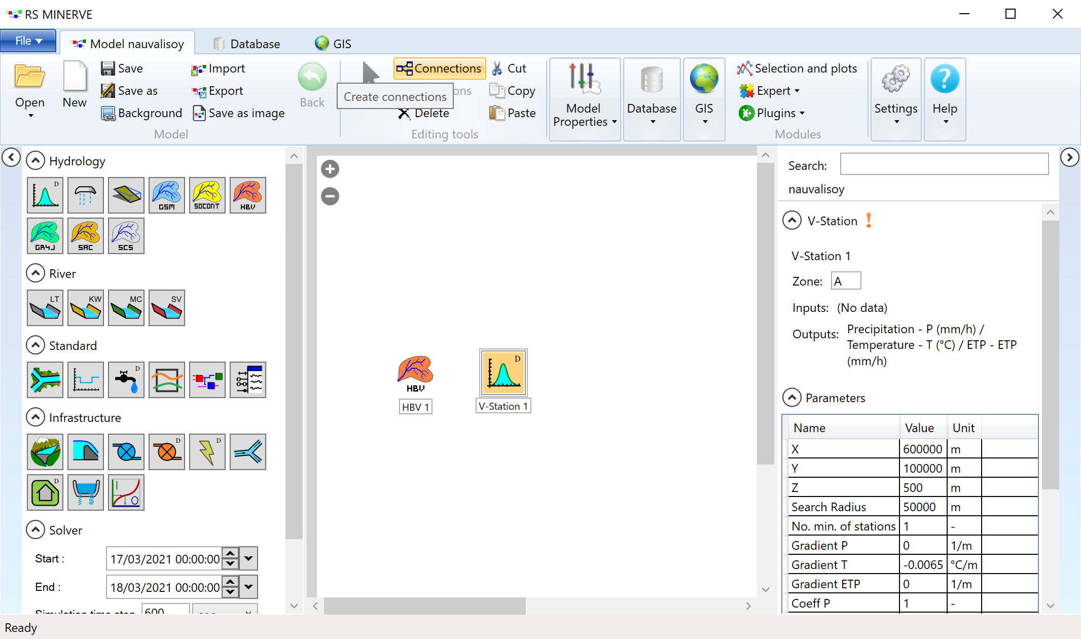
RSM: Add and link climate station
Move your cursor to the V-Station icon in the models panel (the first icon in Figure C.54). Click on the icon to activate it and click next to the HBV model in your model pane to place the V-Station. With a double-click on the newly created V-Station, you can visualize the parameters of the virtual weather station.
Then, connect the station to the HBV model by activating the Connections Mode in the Editing tools toolbar as shown in Figure C.60.
Click on the station, hold down the finger move your cursor to the HBV model, then release the hold. A grey line appears between the station and the model and a pop-up window asks you to verify the data links between the two components (see Figure C.61).
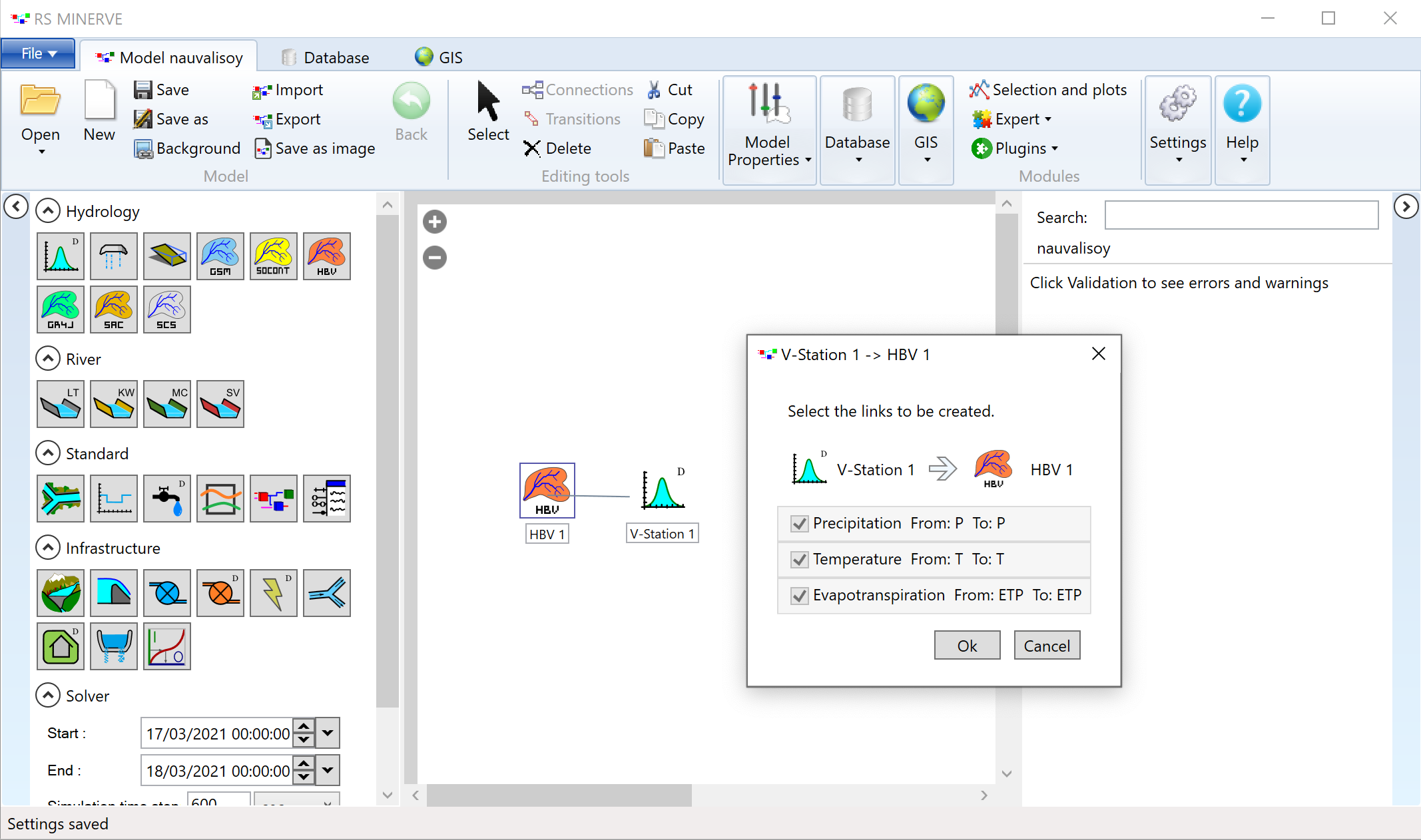
Click Ok to accept the suggested data links and a blue arrow will appear between the weather station and the model. Click on the black arrow in the Editing tools toolbar to leave the Connections Mode.
Back to the Nauvalisoy model guide.
RSM: Import climate data
Make sure that you have downloaded storede the following climate data file ERA5_Nauvalisoy_1981_2013.csv for Nauvalisoy River on your computer.
Go to the database tab and click on Open in the File database toolbar (see Figure C.62).
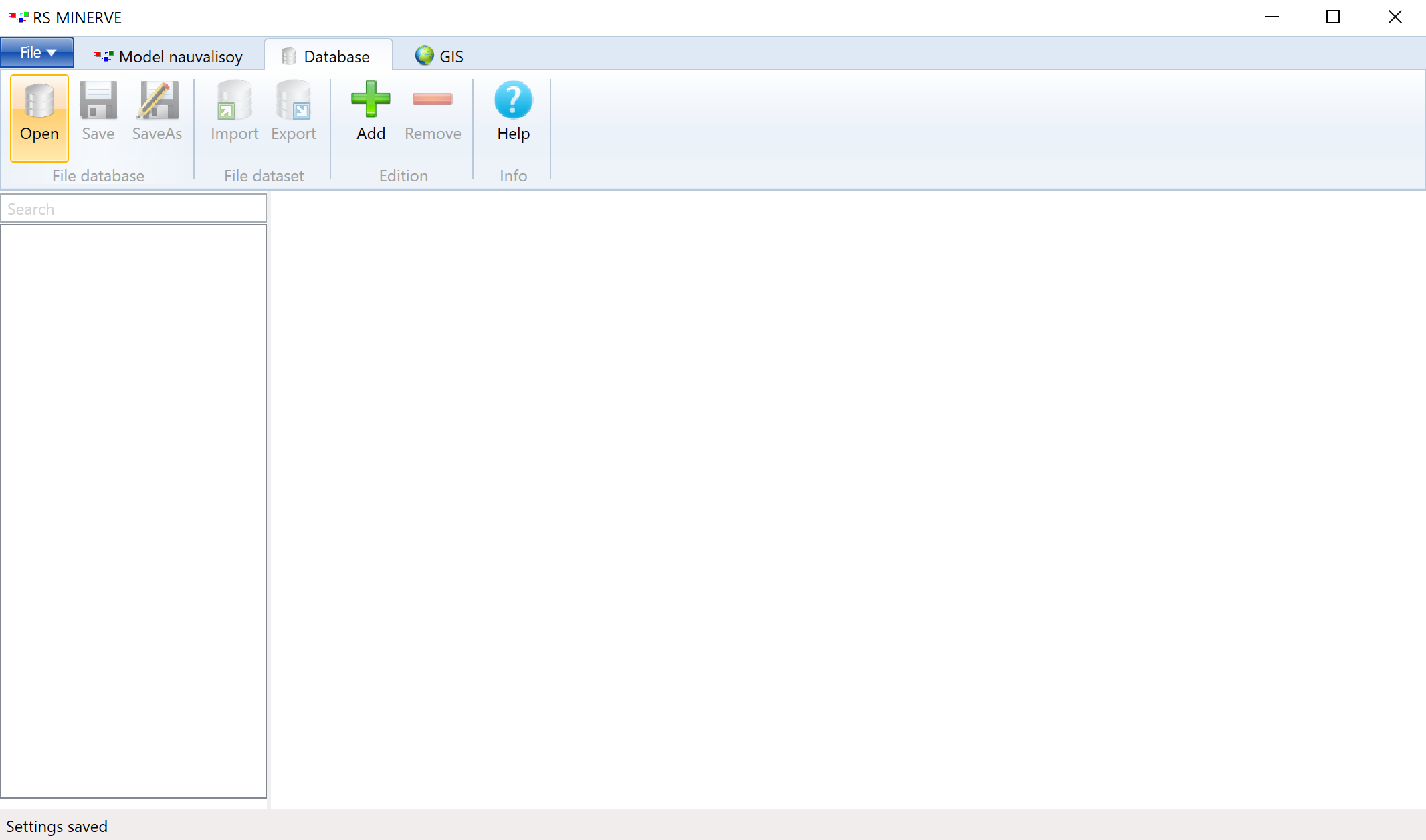
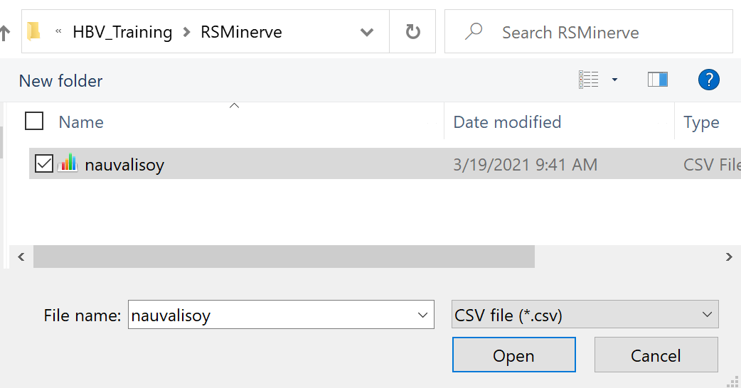
Select the file that you downloaded before. If you don’t see the file in your file browser, make sure the file ending .csv is selected in the file browser (see Figure C.63).
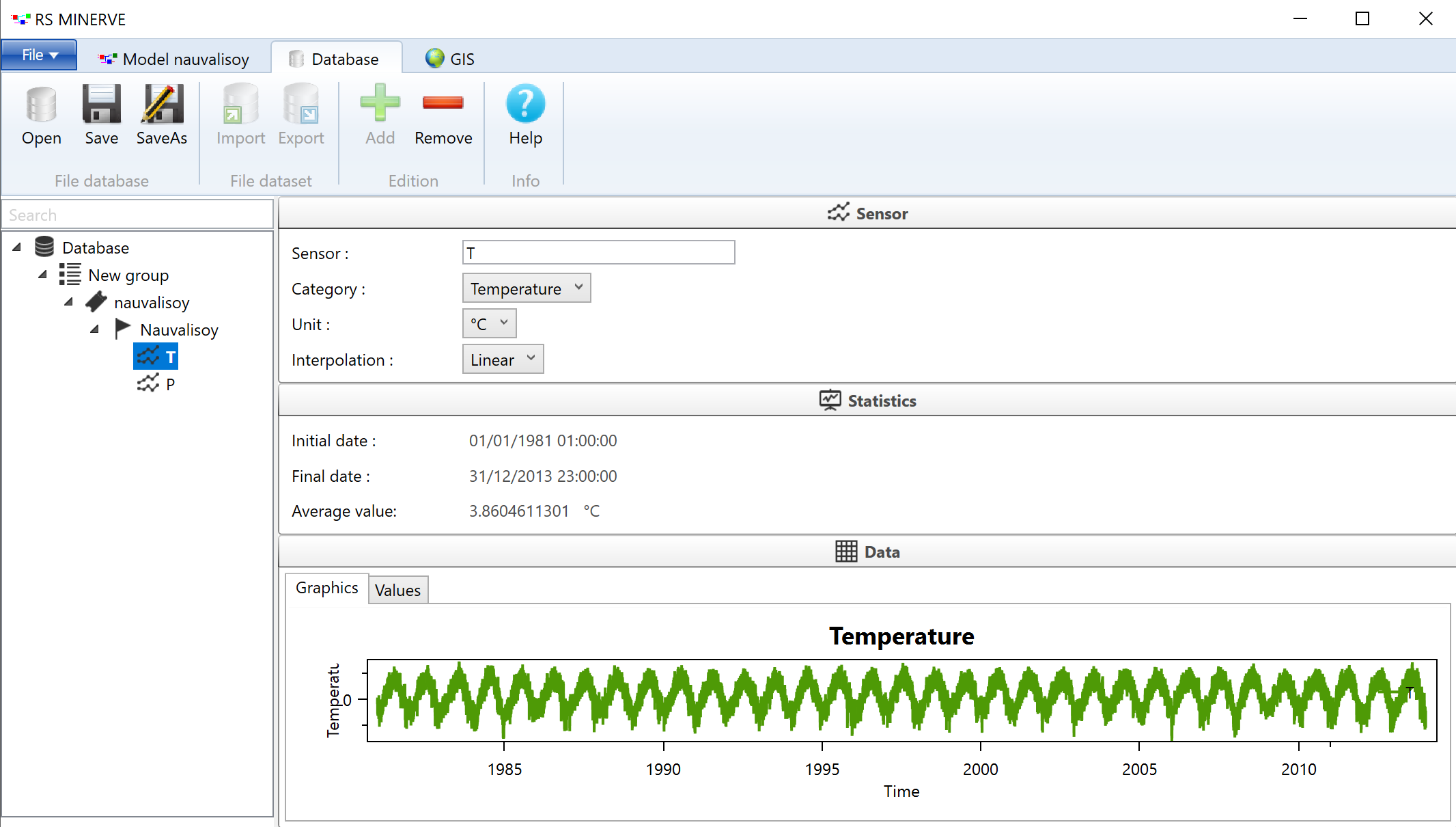
Press open to load the data into RSMinerve. Depending on your computer this may take a few seconds. Once the data is loaded, click through the database browser in the left pane to explore the data as shown in Figure C.64.
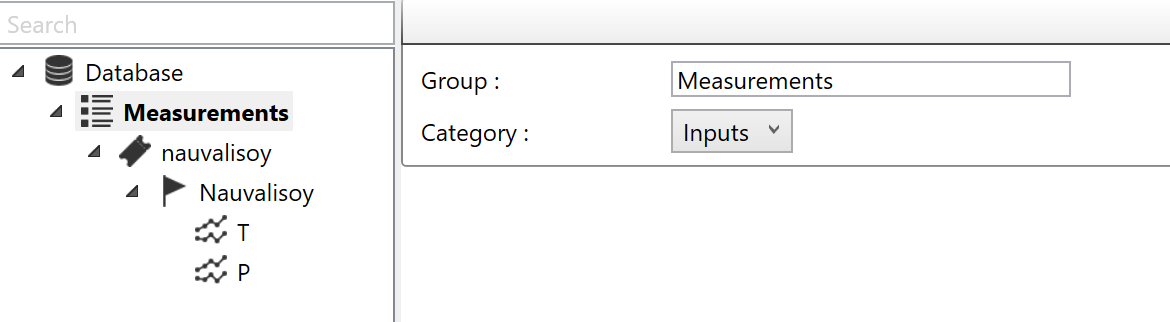
To connect the data base to the model you will need to make the data consistent with the model. To do this change the name “New group” to “Measurements” and select Inputs for the Category selection (see Figure C.65).
Then, browse the name of the station as done in Figure C.66.
As our weather data is representative for the entire Nauvalisoy catchment, the station name in the data base needs to be consistent with the station name of the V-Station in the model pane. Change the name of the station in the model pane from V-Station to Nauvalisoy by clicking on the name and then editing it.
Choose the nauvalisoy data set as source and adapt the simulation period as shown in Figure C.67.
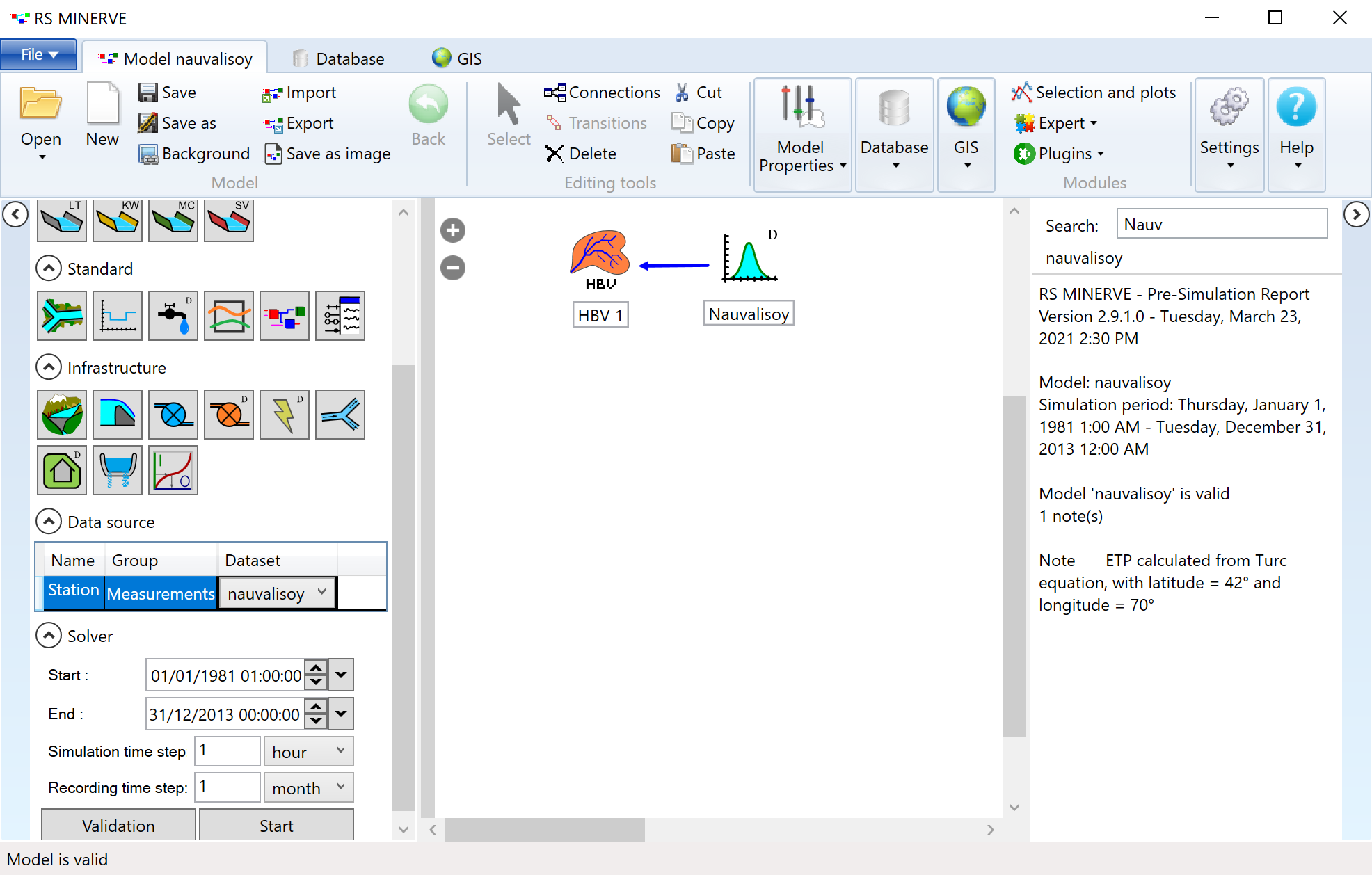
Click on Validation to verify that the model has been set up correctly. Once you have adapted the model settings to calculate evaporation based on temperature (how to), no errors should be reported. You can now run the model. A warning tells you that the number of meteo stations is not sufficient. Ignore the warning for now.
Back to the Nauvalisoy model guide
RSM: Adapt Model Settings
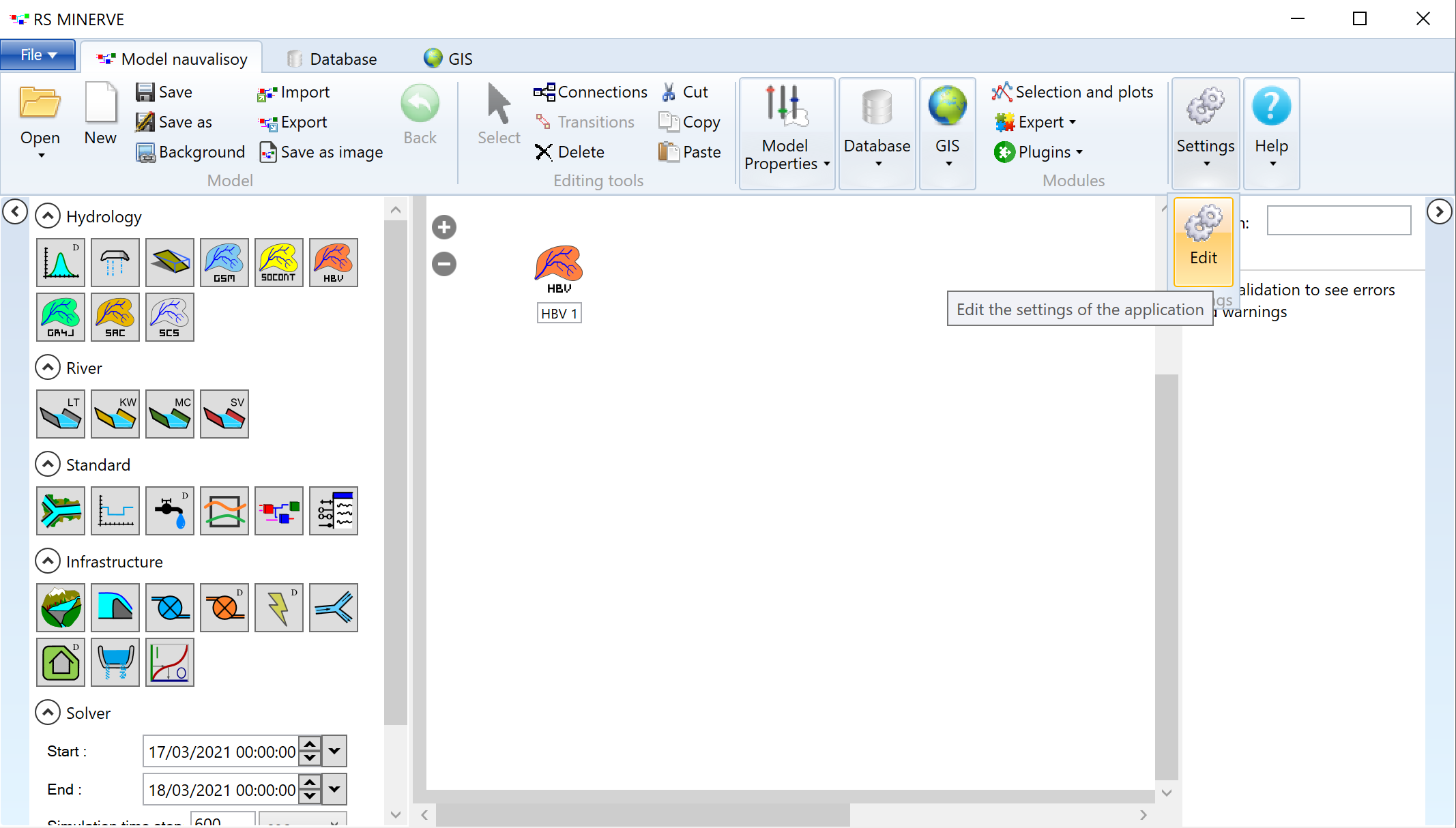
Navigate to Edit in the Settings toolbar (see Figure C.68).
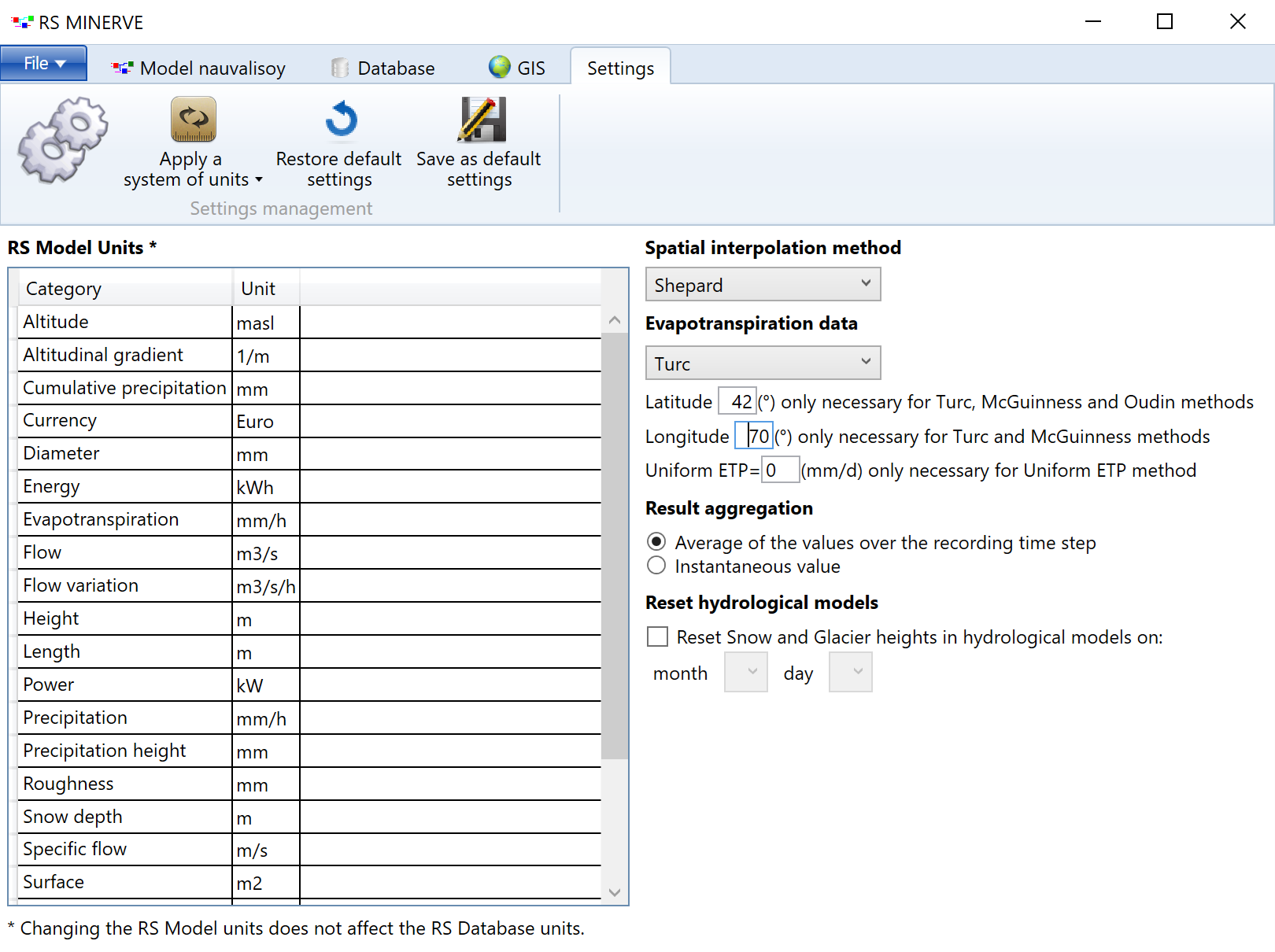
Open the Settings tab and choose an ET model. Adapt the coordinates of the project (choose the station coordinates mentioned in the Introduction Section) (see Figure C.69).
Back to the model guide
RSM: Export Simulation Results to Data Base
Go to Export in the Database toolbar (see Figure C.70). Define a name for the simulation results and choose a data base group to save the data to. Create a new group if you haven’t already done so.
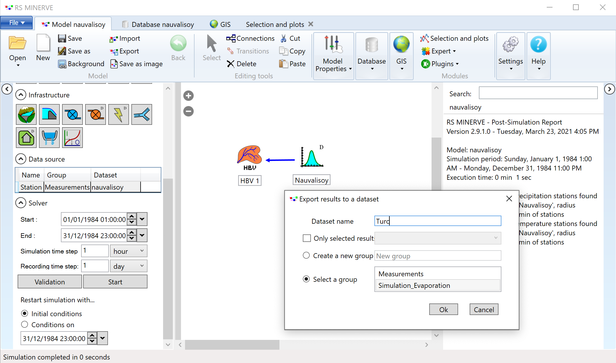
The data sets are now available in the data base tab and can be visualized in the Selection and Plots tab.
Back to the model guide
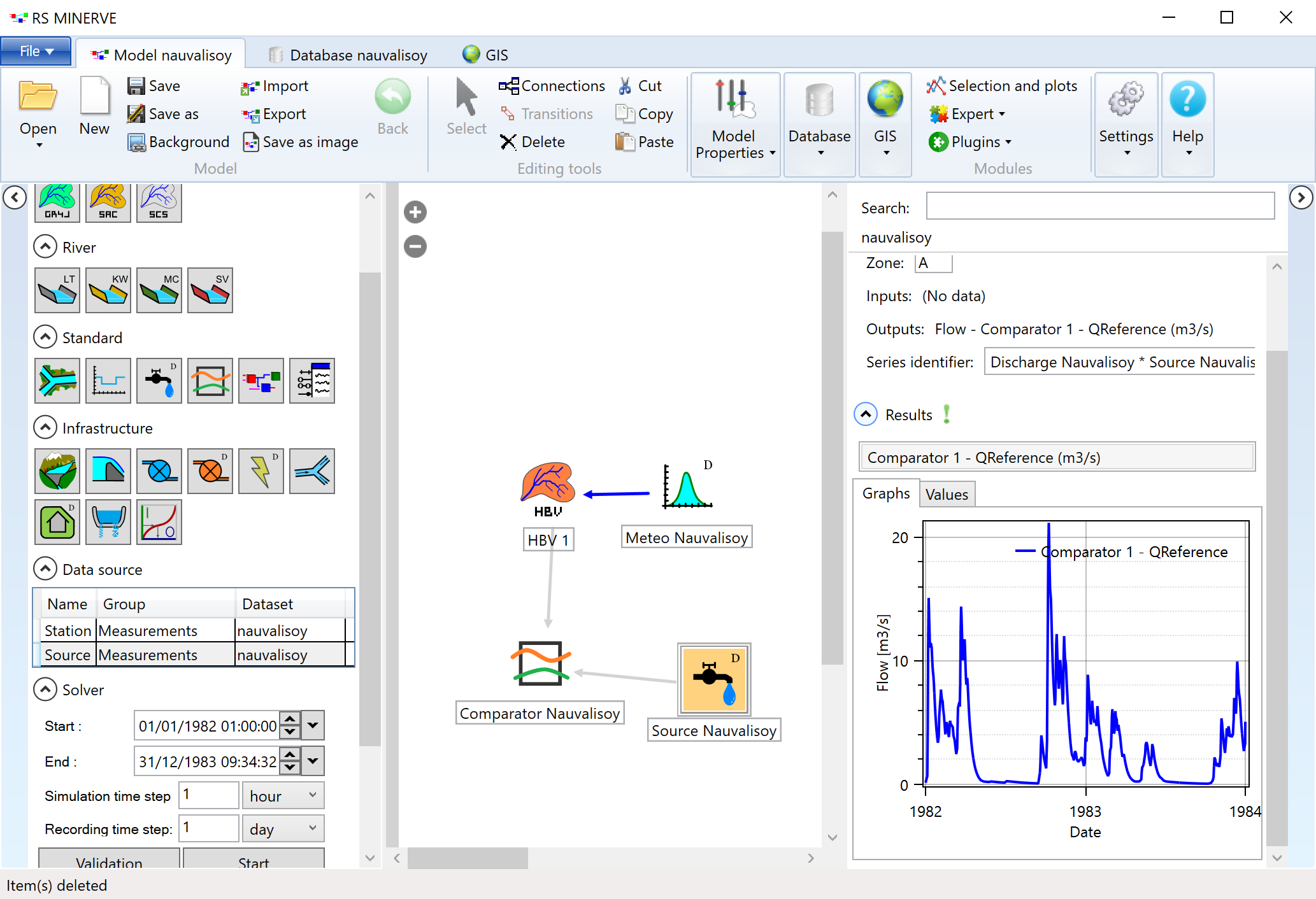
RSM: Add Comparator and Load Discharge Measurements
The comparator object allows the user to compare a simulated variable to a reference. In our case, we want to compare the simulated discharge of the Nauvalisoy river to the one actually measured at the only gauge in the catchment. The measured discharge can be imported to RSMinerve via the database tab.
Move your cursor to the comparator icon as shown in Figure C.71 in the model components panel.
Activate it with a left-click and move your cursor next to the HBV model in the model pane. Place the comparator object with another click.
Add a source object to your model following the same procedure as for the comparator object. Figure C.72 shows the icon of the source object.
You can now optionally rename your model objects.
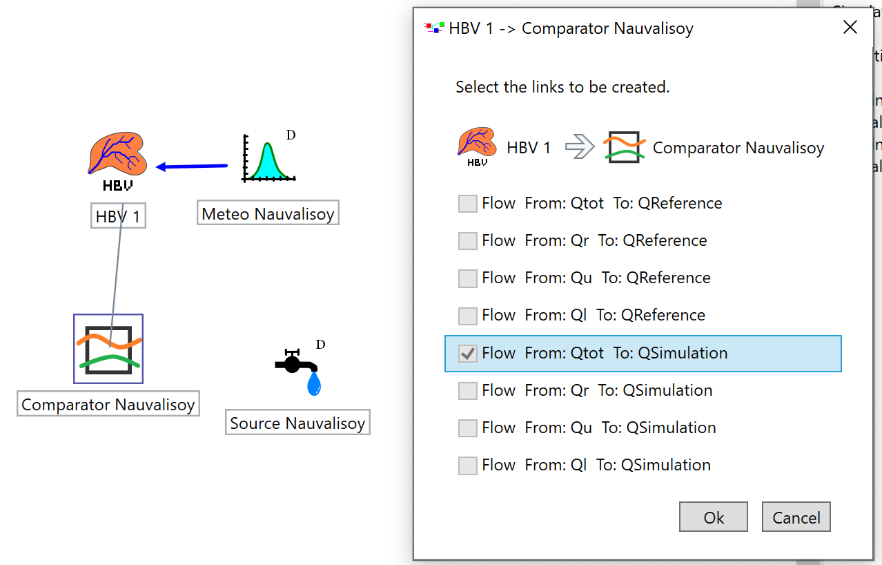
Connect the source and the HBV model to the comparator by activating the Connections mode in the Editing Tools toolbar. Right-click on the HBV model, hold the click and drag the cursor to the comparator object where you release the cursor. You will be asked in a pop-up window to specify the flow you wish to compare and if the data is to be viewed as simulation results or reference (measured) data. Connect the total discharge computed by the HBV model component as simulation result to the comparator (see Figure C.73) and close the pop-up window by pressing OK.
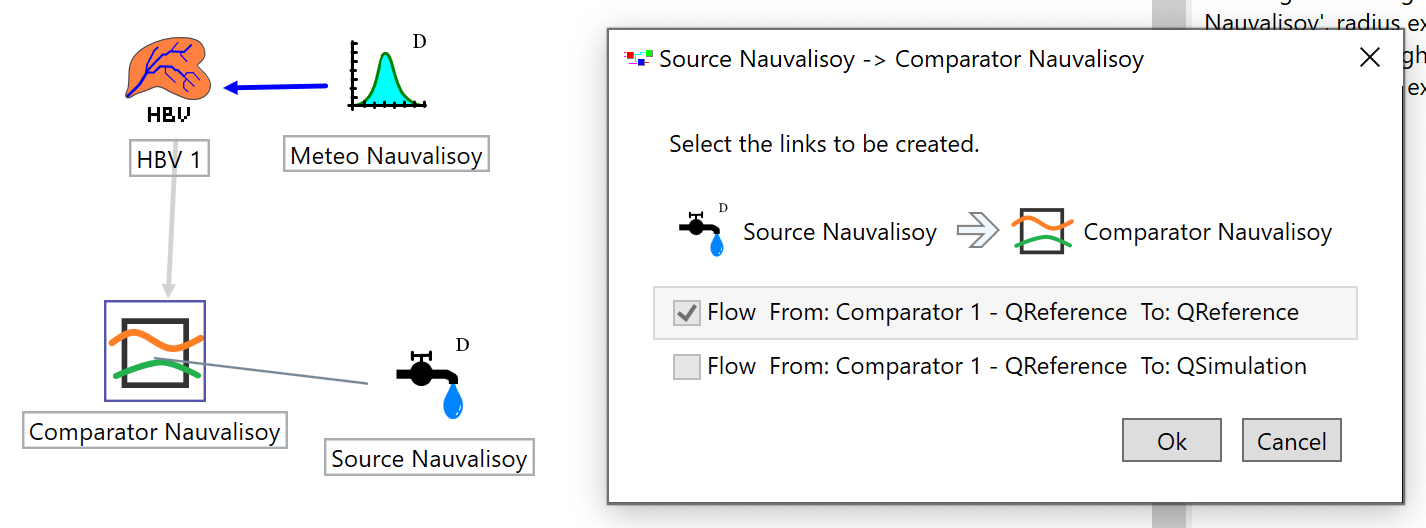
Connect the source object to the comparator in the same way as the HBV object. The source will be connected as reference (see Figure C.74).
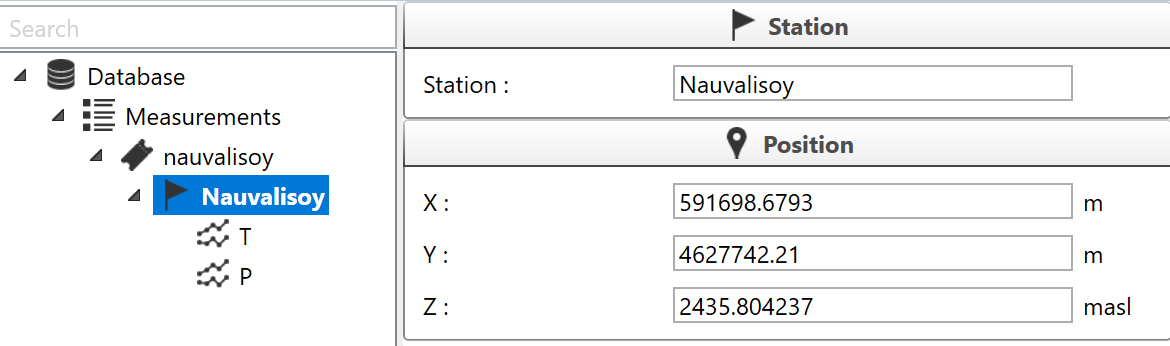
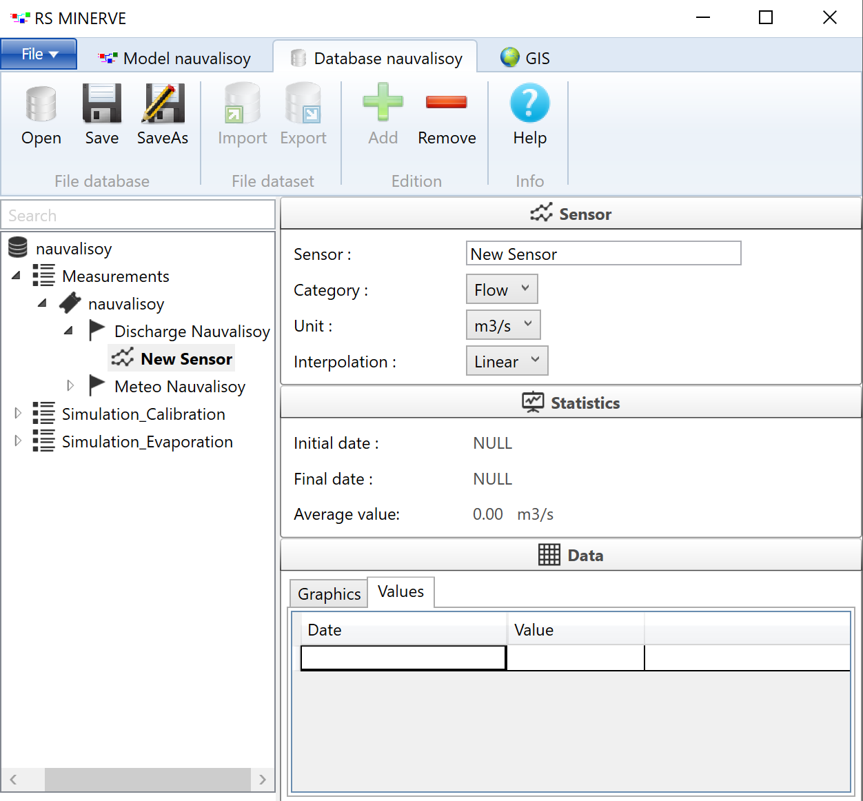
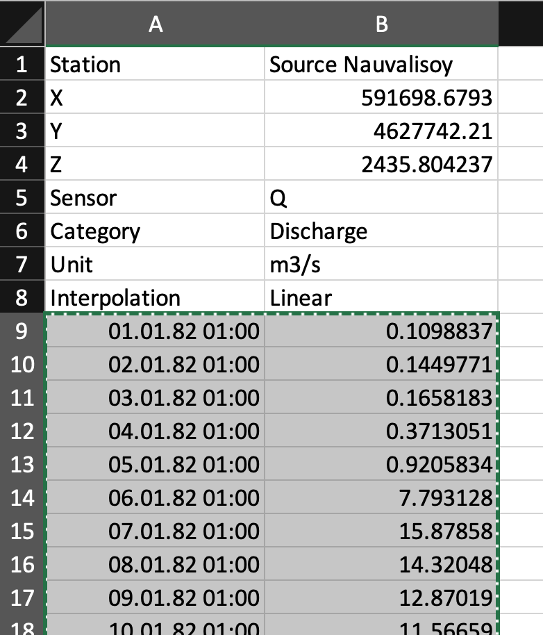
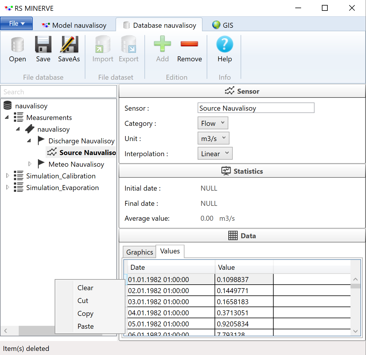
Next, we have to load the discharge data into the database. Navigate to the database tab. In the database, go to Measurements -> Nauvalisoy and click Add and enter a name for the discharge station (see Figure C.75). For this example, we do not need to bother with the coordinates of the station (later, in more complex models, we will have to though!).
Under the new discharge station, add a sensor and rename it to the source object in your model as shown in Figure C.76.
Open the tab with the values. Here we need to import the discharge data. You can do that by opening the discharge data in a spreadsheet (e.g. Excel) and copy-pasting the dates and discharge values into the Values table in RSMinerve (here is how to do this step-by-step.
Now we need to link the discharge data in the database to the source object in the model. Navigate to the model do the following.
Validate the model to see if the model setup went correctly. Run the model if the validation did not throw an error.
Back to the practical model calibration and validation Section
RSM: Copy-paste Data to Database
Make sure that the following file synthetic_discharge_Nauvalisoy_river_for_calibration_exercise.csv is available on your computer.
Now, open the file in a spreadsheet software, e.g. Excel, Numbers, Google Sheets or OpenOffice Calc and select the rows containing dates and values (Figure C.78). Press Control+C or perform a right-click with the mouse and choose copy.
Then navigate to the discharge sensor on the database tab in RSMinerve where you want to add the data to. Click in the small square to the left of the first row in the Values tab and click the keyboard keys Control+P. Alternatively perform a right-click in the small square and select Paste. The dates and values from the excel sheet will now appear in the table (Figure C.79). Save the database.
Back to the practical model calibration and validation Section