Simulating the Shakhimardan catchment
This example simulates discharge of the Shakhimardan catchment, a left tributary of the Syr Darya in the Ferghana valley.
Check out the on-line book Applied Modeling of Hydrological Systems in Central Asia for descriptions of how to set up a hydrological model in RSMinerve and the R package riversCentralAsia for helpful functions.
The data for this vignette are available in the on-line repository. This vignette will attempt to download the required files to a local folder.
Prerequisites
Install R, RTools, RStudio, RSMinerve and the R package rClr (see README for instructions and links).
Copy this vignette to your local computer and adapt the paths.
Open the model in and load & link the data base with the model objects. If you don’t know how to do this please follow the examples in the RS Minerve User Manual prior to continuing with this tutorial.
Open the Selection and plots tab by clicking on its icon
in the in the modules toolbar. Define a selection of model results to
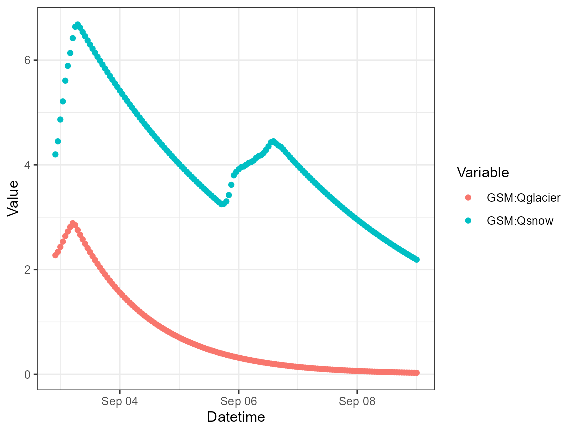
visualize (here we define two result groups:
DischargeGlacier and SnowWaterEquivalent. Save
the model.
Loading Assemblies
# Adapt path in dir_RSM_install to your local installation of RSMinerve.
dir_RSM_install <- "C:/Program Files (x86)/RS MINERVE"

clrLoadAssembly(file.path(dir_RSM_install, 'log4net.dll'))
clrLoadAssembly(file.path(dir_RSM_install, 'Microsoft.Practices.Prism.Mvvm.dll'))
clrLoadAssembly(file.path(dir_RSM_install, 'RSMinerve.RS.dll'))
clrLoadAssembly(file.path(dir_RSM_install, 'RSMinerve.DB.dll'))
clrLoadAssembly(file.path(dir_RSM_install, 'RSMinerve.Base.dll'))
Model settings
model_file <- if (file.exists("../inst/extdata/Tutorial_Model.rsm")) {
   "../inst/extdata/Tutorial_Model.rsm"
} else {
  "https://raw.githubusercontent.com/hydrosolutions/RSMinerveR/main/inst/extdata/Tutorial_Model.rsm"
}

input_dataset <- if (file.exists("../inst/extdata/Tutorial_DataMeteo.dsx")) {
   "../inst/extdata/Tutorial_DataMeteo.dsx"
} else {
  "https://raw.githubusercontent.com/hydrosolutions/RSMinerveR/blob/main/inst/extdata/Tutorial_DataMeteo.dst"
}

parameter_file <- if (file.exists("../inst/extdata/Tutorial_Parameters.txt")) {
   "../inst/extdata/Tutorial_Parameters.txt"
} else {
  "https://raw.githubusercontent.com/hydrosolutions/RSMinerveR/blob/main/inst/extdata/Tutorial_Parameters.txt"
}

results_previous <- if (file.exists("../inst/extdata/ResultsPrevious.dsx")) {
  "../inst/extdata/ResultsPrevious.dsx"
} else {
  "https://raw.githubusercontent.com/hydrosolutions/RSMinerveR/blob/main/inst/extdata/ResultsPrevious.dst"
}

saveDataInDstFile <-  TRUE

# The RS Minerve documentation describes the date format to be "%d.%m.%Y"
start_date <- "02.09.2013 00:00:00"  # format = "%d.%m.%Y %H:%M:%S"
end_date <- "09.09.2013 00:00:00"  # format = "%d.%m.%Y %H:%M:%S"

simulationTimeStep <- "600"
recordingTimeStep <- "3600"
timeStepUnit <- "Seconds"
The paths for the result files need to be full paths. Below are example paths. You’ll need to adapt these.
results_savePath <-
  "C:/Users/<username>/Documents/scriping_rsm/tutorial05-results.dsx"
presimreport_path <-
  "C:/Users/<username>/Documents/scriping_rsm/tutorial05-preSimuReport.txt"
postsimreport_path <-
  "C:/Users/<username>/Documents/scriping_rsm/tutorial05-postSimuReport.txt"
Applying settings and running the model
The commands allow to call the Visual Basics commands documented in the RS Minerve Technical Manual. The calls return NULL when successful. Check your local paths to see if the output files have been created.
# Define a clr task
rsm <- clrNew("RSMinerve.RS.Task")

# Start-up the model
clrCall(rsm, "Start", model_file)
#> NULL

# Load data
clrCall(rsm, "LoadDatasetAndSetDates", input_dataset, TRUE, TRUE)
#> NULL

# Get dates from previous and current simulation and check validity
EndDatePrevious = clrCall(rsm, "GetEndDateFromDataset", results_previous, TRUE)
StartDateNew = clrCall(rsm, "GetStartDateFromModel")
EndDateNew = clrCall(rsm, "GetEndDateFromModel")

if (EndDatePrevious >= StartDateNew & EndDatePrevious < EndDateNew) {
  clrCall(rsm, "SetStartDate", format(EndDatePrevious, format = "%d.%m.%Y %H:%M:%S"))
} else {
  cat("Error: EndDatePrevious not within simulation period. ")
  clrCall(rsm, "Stop")
}
#> NULL

# SetSimulationTimeStep and SetRecordingTimeStep require characters
clrCall(rsm, "SetSimulationTimeStep", simulationTimeStep, timeStepUnit)
#> NULL
clrCall(rsm, "SetRecordingTimeStep", recordingTimeStep, timeStepUnit)
#> NULL

# Load IC from previous simulations
clrCall(rsm, "LoadInitialConditionsFromDataset", results_previous)
#> NULL

# Load parameters from file
clrCall(rsm, "LoadParametersFromFile", parameter_file)
#> NULL

# Write a pre-simulation report to check for possible errors (requires full
# path)
clrCall(rsm, "SavePreSimulationReportAs", presimreport_path)
#> NULL

# Run a simulation
clrCall(rsm, "Simulate")
#> NULL

# Write a post-simulation report to check for possible errors (requires full
# path)
clrCall(rsm, "SavePostSimulationReportAs", postsimreport_path)
#> NULL

# Save results (requires full path)
clrCall(rsm, "SaveFullResultsAs", results_savePath, saveDataInDstFile)
#> NULL

# Stop task
clrCall(rsm, "Stop")
#> NULL
Read results
# Calculate the number of time steps to read for each model component, i.e. the
# chunk size. Including the header of each chunk.
chunk_size <- getChunkSize(
  lubridate::as_datetime(EndDatePrevious),
  lubridate::as_datetime(end_date, format = "%d.%m.%Y %H:%M:%S"),
  recordingTimeStep
)
result <- readResultDST(results_savePath, chunk_size)