Background & Motivation
In the Central Asia region, there are key figures to keep in mind in relation to runoff formation: Snow melt is the most important contribution to discharge (~ 80 %, on average), followed by runoff from liquid precipitation (~ 17 %, on average) and, finally, glacier melt (~ 3 %, on average) (personal communication with A. Yakovlev, 2019). Armstrong et al. (2019) obtain similar orders of magnitude with 65%-75% snow melt, 23% precipitation and 2-8% glacier melt for the basins of the rivers Syr Darya and Amu Darya. In smaller, highly glaciated catchments, the glacier contribution to discharge can be more important (Pohl et al. 2017; Dhaubanjar et al. 2021). The cryosphere is therefore a major contributor to the water balance in Central Asia (Barandun et al. 2020). While glacier runoff is a small contributor to the annual runoff, it is seasonally important as it covers the irrigation demand in summer, when snow melt is over (Kaser, Grosshauser, and Marzeion 2010). Gaining a proper understanding of climate change impacts on the region’s hydrology is not just of interest to the scientific community but also of greatest relevance to the local communities and riparian states that depend crucially on the availability of runoff at the right time and location.
Among other things, climate impacts translate into long-term changes of runoff formation fractions and the distribution of runoff formation within the hydrological year. Typical rainfall-runoff models such as the HBV Model simulate the fractionation of precipitation into snow and rain with a temperature threshold method. Snow and liquid water reservoirs and corresponding fluxes are then accounted for. However, these models have only a limited understanding of glacier processes which are normally inadequate at best to estimate glacier contributions to discharge. We present a short introduction to glaciers in water resources and a workflow to include state-of-the-art glacier data from the scientific community in day-to-day hydrological modelling.
Glaciers in Water Resources Modelling
Glaciers consist of compacted snow and frozen water. Many processes contribute to the glacier mass balance (see for example Benn and Evans (2010) and Cogley et al. (2011)) but we focus on a simplified mass balance as we have data only for accumulated mass balance outcomes (i.e. glacier thinning rates and glacier discharge, see below).
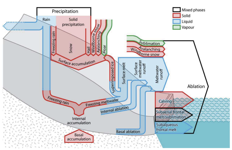
Glacier mass balance components (thickness of arrows not to scale) by Cogley et al. (2011).
Glaciers accumulate mass in the cold period and at higher altitudes through snow fall. Glaciers lose mass to melt driven by the energy balance at the glacier-atmosphere interface (Hock 2005). Typically, larger glaciers loose mass at lower altitudes (ablation zone) and accumulate mass at higher altitudes (accumulation zone). The mass loss in the lower altitudes is compensated by the downstream movement of ice from the accumulation zone. The boundary between the accumulation and the ablation zone is called the equilibrium line altitude (ELA).
Naturally, glaciers accumulate mass in the cold season and loose mass to ablation in the warm season. Therefore, the overall mass balance of a glacier should be calculated over a year or, better, over an average of several years.
A simplified multi-year average glacier mass balance, neglecting snow melt, can be expressed as (Braithwaite and Zhang 2000):
\[ \Delta S = \text{accumulation} - \text{ablation} \approx P - M \]
where \(\Delta S\) is the change of water storage in the glacier, \(P\) is the precipitation over the glacier (assumed to be solid precipitation) and \(M\) is glacier melt. If \(\Delta S\) is larger than 0 (i.e., \(P > M\)), the glacier accumulates snow and ice and is growing. If \(\Delta S\) is smaller than 0 (i.e., \(P < M\)), we have imbalance ablation and the glacier shrinks.
Glacier melt \(M\) can be modeled using full energy balance models or simplifications thereof, e.g. temperature index models (Hock 2003).
In simplified words, if a glacier, on average, accumulates as much snow as it looses to melt, it is in balance. The average annual glacier discharge is equivalent to the average annual snow fall and called balance ablation. The ELA does not move. If the glacier produces more discharge than it accumulates from snow fall, it is not in balance. The ELA moves upwards. The excess melt is called imbalance ablation, as also explained in the previous paragraph. If more snow falls that melts, the ELA moves downstream and the glacier grows (Cogley et al. 2011).
Glacier graphics by Anne Maussion, Atelier les Gros yeux, for Open Global Glacier Model (OGGM).
Most glaciers worldwide are currently not in equilibrium with the warmer than long-term average climate and thus produce excess melt via imbalance ablation (Hugonnet et al. 2021). In the short term, this is for example good in semi-arid places such as Central Asia where more river discharge is temporarily available in the downstream for irrigation. However, the glaciers produce excess melt only until they reach a new equilibrium at higher altitudes or until they disappear entirely. This means that the excess melt will also disappear and ultimately less water will be available for downstream users during the warm season where glaciers contribute most to runoff. This phenomenon is called peak water (Huss and Hock 2018).
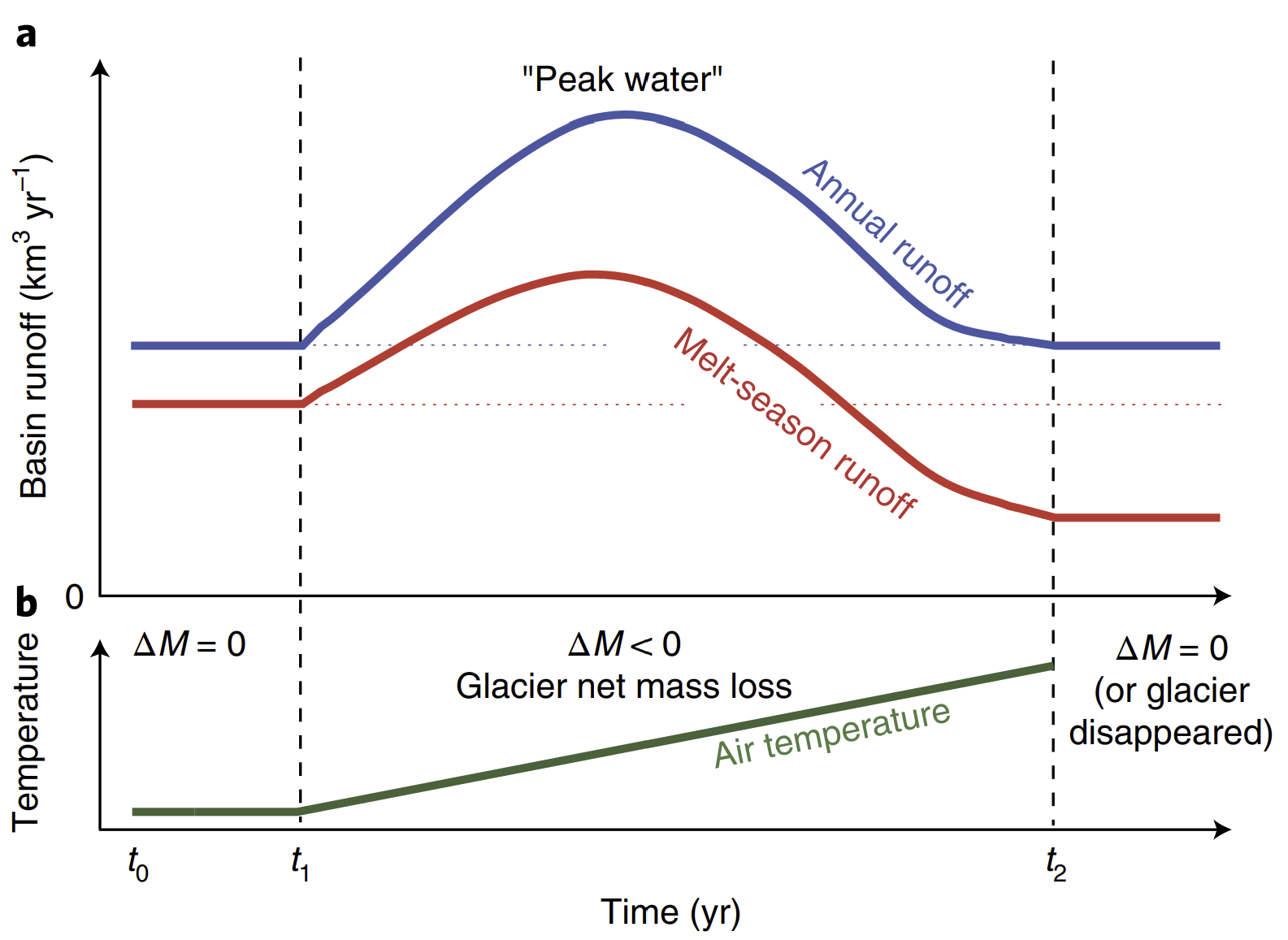
An illustration of peak water by Huss and Hock (2018).
Water resources managers in glaciated catchments are highly interested in knowing when peak water will be reached as measures to adapt for lower water availability need time to implement.
Without in-situ measurements (and actually even with in-situ measurements) it is no easy feat to model the evolution of the water storage in a glacier. The best we can do in water resources modelling is: Use results from existing glacier models and feed them to the water resources model or, alternatively, use the best data available to estimate glacier melt with simple models. As state-of-the-art glacier models are available as open source software (Maussion et al. 2019; Rounce, Hock, and Shean 2020a), and even simulation results are published for public use (Rounce, Hock, and Shean 2020a), there is no need to implement an own glacier evolution model. New glacier thickness data sets can be used to update glacier-volume scaling relationships derived for glaciers in Central Asia.
The present vignette gives an overview over the relevant glacier-related data, illustrated using the catchment area of the river Atbashy, a tributary of the Naryn river in Central Asia (status mid 2022).
Availability on glacier-related data
Recent advances in glacier research yielded a stupendous amount of novel data sets that can be used to map glaciers and to force glacier melt models. The following section gives an overview over the data used in the models, status January 2022.
We use the catchment of the gauging station on the Atabshy river, a tributary to the Naryn river in Central Asia as a demo site. If you’d like to reproduce the examples presented in this vignette you can download the riversCentralAsia_ExampleData (see README). The rest of the code will run as it is, provided you have the required r packages installed. The size of the data package is approximately 1 GB.
# Install the libraries required to reproduce this vignette
# The below packages are available from cran and can be installed using the
# command install.packages. Example: install.packages("tmap")
library(tmap)
library(sf)
library(raster)
library(tidyverse)
library(lubridate)

# The package riversCentralAsia is not available from cran. It is installed
# directly from github via:
devtools::install_github("hydrosolutions/riversCentralAsia")
# Make sure to update the package from time to time as it is under constant
# development.
library(riversCentralAsia)

data_path <- "../../riversCentralAsia_ExampleData/"
Randolph glacier inventory
The Randolph Glacier Inventory (RGI) v6.0 (RGI Consortium 2017) makes a consistent global glacier data base publicly available. It includes geo-located glacier geometry and some additional parameters, for example elevation, length, slope and aspect. A new version (v7) is under review at the time of writing mid 2022. For Central Asian water resources modelling, RGI regions 13 (Central Asia) and 14 (South Asia West) are relevant. You can download the glacier geometries for all RGI regions from the GLIMS RGI v6.0 web site. For this demo, the data is available from the data download link given above.
dem <- raster(paste0(data_path, "16076_DEM.tif"))
basin <- st_read(paste0(data_path, "16076_Basin_outline.shp"), quiet=TRUE)

rgi <- st_read(paste0(data_path, "16076_Glaciers_per_subbasin.shp"),
               quiet = TRUE) |>
  st_transform(crs = crs(dem))

tmap_mode("view")
tm_shape(dem, name = "DEM") +
  tm_raster(n = 6,
            palette = terrain.colors(6),
            alpha = 0.8,
            legend.show = TRUE,
            title = "Elevation (masl)") +
  tm_shape(rgi, name = "RGI v6.0") +
  tm_polygons(col = "lightgray", lwd = 0.2) +
  tm_scale_bar(position = c("right", "bottom"))
Note: The python package rgitools provides functions pre-processing RGI glacier outlines, such as automated data quality checks or glacier hypsometry data1.
Glacier thickness
Two global glacier thickness datasets are currently publicly available: Farinotti et al. (2019a) and Milan, Mouginot, and Rabatel (2021).
Farinotti et al. (2019b) make distributed glacier thickness maps available for each glacier in the RGI v6 data set as individual tifs. Millan et al. (2022) provide one tif for each RGI region which is more convenient to handle.
thickness <- raster(paste0(data_path,
                           "Milan_glacier_thickness.tif"))

values(thickness)[values(thickness) <= 0] = NA

tmap_mode("view")
tm_shape(dem, name = "DEM") +
  tm_raster(n = 6,
            palette = terrain.colors(6),
            alpha = 0.8,
            legend.show = TRUE,
            title = "Elevation (masl)") +
  tm_shape(thickness, name = "Thickness") +
  tm_raster(n = 6,
            palette = "Blues",
            title = "Thickness [m]") +
  tm_scale_bar(position = c("right", "bottom"))
Glacier area-volume scaling
Well-established methods exist to derive the outlines of glaciers from remote sensing data (RGI Consortium 2017), i.e. the glacier areas are relatively well known (on a global scale). Until recently, glacier volumes have not been available to the wider public and scaling relationships have been used to derive glacier volumes based on glacier area or length, for example (Bahr, Meier, and Peckham 1997; Van de Wal and Wild 2001; Radić and Hock 2006). And although these scaling relationships have been derived from glaciers presumably in steady-state conditions, Radić, Hock, and Oerlemans (2007) have found it to be suitable for long-term glacier development. In Central Asia, the scaling relationship by Erasov (1968) is the most widely applied method, an empirical function of the form:
\[ V = a \cdot A^{b} \]
With \(a=0.027\) and \(b=1.5\). Using the RGI v6.0 glacier outlines of region 13 (Central Asia) and the glacier thickness data set by Farinotti et al. (2019b), the volume of each glacier can be estimated and the area-volume scaling by Erasov (1968) can be validated (see CAHAM book). While the relationship derived by Erasov is still valid for glaciers below 20 km2, it may overestimate the glacier volume of larger glaciers. Using the novel data, the parameters of the empirical scaling function derived by Erasov (1968) can be updated to \(a=0.0388\) and \(b=1.262\) to form what we call the RGIF scaling relationship.
The scaling relationship can be inverted to derive glacier areas based on glacier volumes as:
\[ A=\exp{\left(\frac{\left(\log{V} - \log{a}\right)}{b}\right)} \]
The package riversCentralAsia implements the area-volume
scaling and the volume-area scaling with parameter sets from Erasov and
derived from RGI Consortium (2017) and
Farinotti et al. (2019b) in the functions
glacierArea_Erasov(), glacierArea_RGIF(),
glacierVolume_Erasov() and
glacierVolume_RGIF().
Further scaling functions to derive glacier area and volume based on
glacier length have been published by Aizen,
Aizen, and Kuzmichonok (2007). These empirical equations have
been derived for glaciers in the Tien Shan mountains and are implemented
as glacierAreaVolume_Aizen() in the riversCentralAsia
package. Aizen computes glacier Area \(A\) from glacier length \(L\) as follows:
\[A=\left(\frac{L}{1.6724}\right)^{\frac{1}{0.561}}\]
And glacier volume \(V\) depeding on glacier area:
\[V=0.03782 \cdot A^{1.23}\text{ }\text{ }\text{ for }\text{ }\text{ } A<0.1\text{ km}^2\]
\[V=\frac{\left(0.03332 \cdot A^{1.08} \cdot e^{0.1219 \cdot L}\right)}{L^{0.08846}}\text{ }\text{ }\text{ for }\text{ }\text{ } 0.1 < A < 25\text{ km}^2\]
\[V=0.018484 \cdot A + 0.021875 \cdot A^{1.3521}\text{ }\text{ }\text{ for }\text{ }\text{ } A > 25\text{ km}^2\]
Glacier runoff
Rounce, Hock, and Shean (2020a) published simulated projections of glacier runoff from till 2100 for the average over the CMIP5 GCM model ensemble2 and for all RCPs3. They used the model PyGEM (Python Glacier Evolution Model) which is available via GitHub. The data can be accessed from Rounce, Hock, and Shean (2020b).
Further data that can be used for cross-validation
Glacier thinning rates
Hugonnet et al. (2021) provide annual estimates of glacier thinning rates for each glacier in the RGI v6.0 data set. A copy of the Hugonnet thinning rates is included in the download link above.
The per-glacier time series of thinning rates is available from the data repository as described in the github site linked under the code availability section of the online paper of Hugonnet et al. (2021). The data is available in a compressed format and you will have to extract it before you can use it.
hugonnet <- read_csv(paste0(<path to your copy of the Hugonnet data>,
                            "dh_13_rgi60_pergla_rates.csv"))

# Explanation of variables:
# - dhdt is the elevation change rate in meters per year,
# - dvoldt is the volume change rate in meters cube per year,
# - dmdt is the mass change rate in gigatons per year,
# - dmdtda is the specific-mass change rate in meters water-equivalent per year.

# Filter the basin glaciers from the Hugonnet data set.
hugonnet <- hugonnet |>
  dplyr::filter(rgiid %in% rgi$RGIId) |>
  tidyr::separate(period, c("start", "end"), sep = "_") |>
  mutate(start = as_date(start, format = "%Y-%m-%d"),
         end = as_date(end, format = "%Y-%m-%d"),
         period = round(as.numeric(end - start, units = "days")/366))

# Join the Hugonnet data set to the RGI data set to be able to plot the thinning
# rates on the glacier geometry.
glaciers_hugonnet <- rgi |>
  left_join(hugonnet |> dplyr::select(rgiid, area, start, end, dhdt, err_dhdt,
                                      dvoldt, err_dvoldt, dmdt, err_dmdt,
                                      dmdtda, err_dmdtda, period),
            by = c("RGIId" = "rgiid"))

tmap_mode("view")
tm_shape(dem, name = "DEM") +
  tm_raster(n = 6,
            palette = terrain.colors(6),
            alpha = 0.8,
            legend.show = TRUE,
            title = "Elevation (masl)") +
  tm_shape(glaciers_hugonnet |> dplyr::filter(period == 20),
           name = "Thinning [m weq/a]") +
  tm_fill(col = "dmdtda",
          n = 6,
          palette = "RdBu",
          midpoint = 0,
          legend.show = TRUE,
          title = "Glacier thinning\n(m weq/a)") +
  tm_shape(rgi, name = "RGI v6.0") +
  tm_borders(col = "gray", lwd = 0.4) +
  tm_shape(basin, name = "Basin outline") +
  tm_borders(col = "black", lwd = 0.6) +
  tm_scale_bar(position = c("right", "bottom"))
Glacier thinning rates can be viewed as net glacier mass change or glacier imbalance ablation (if glacier ice deformation processes are neglected).
Glacier discharge
Miles et al. (2021) ran specific mass balance calculations over many glaciers larger than 2 km2 of High Mountain Asia. They provide the average glacier discharge between 2000 and 2016. A copy of the glacier discharge data is available from the data download link provided above.
The original data is available from the data repository linked in the online version of the paper.
miles <- read_delim(paste0(<path to your copy of Miles glacier ablation rates>,
                           "Miles2021_Glaciers_summarytable_20210721.csv"),
                    show_col_types = FALSE, delim = ",") |>
  dplyr::filter(RGIID %in% rgi$RGIId & VALID == 1)

glaciers_hugonnet <- glaciers_hugonnet |>
  left_join(miles |> dplyr::select(RGIID, totAbl, totAblsig, imbalAbl,
                                   imbalAblsig),
            by = c("RGIId" = "RGIID")) |>
  mutate(Qgl_m3a = ifelse(is.na(totAbl), NA, totAbl))

tmap_mode("view")
tm_shape(dem, name = "DEM") +
  tm_raster(n = 6,
            palette = terrain.colors(6),
            alpha = 0.8,
            legend.show = TRUE,
            title = "Elevation (masl)") +
  tm_shape(glaciers_hugonnet |> dplyr::filter(period == 20),
           name = "Total ablation [m3/a]") +
  tm_fill(col = "Qgl_m3a",
          n = 6,
          palette = "RdBu",
          midpoint = 0,
          legend.show = TRUE,
          title = "Glacier discharge\n(m3/a)") +
  tm_shape(rgi, name = "RGI v6.0") +
  tm_borders(col = "gray", lwd = 0.4) +
  tm_shape(basin, name = "Basin outline") +
  tm_borders(col = "black", lwd = 0.6) +
  tm_scale_bar(position = c("right", "bottom"))
For most hydrological applications, the interest lies on the glacier discharge, i.e. total ablation from glaciers. Despite their large uncertainties, the simulation results by Miles et al. (2021) give us an estimate for glacier melt that we can use to calibrate the simpler temperature index models for glacier melt.
A note on the uncertainties of glacier data sets
The geometries of the RGI v6.0 data set are generally very good. If you simulate glacier discharge in a small catchment with few glaciers it is advisable to visually check the glacier geometries and make sure, all relevant glaciers in the basin are included in the RGI data set. You may have to manually add missing glaciers or correct the geometry.
For some regions in Central Asia, OpenStreetMap is an excellent reference for glacier locations and names in Central Asia. You can import the map layer in QGIS or also download individual.
The glacier thickness data set is validated only at few locations as measurements of glacier thickness are typically not available. Millan et al. (2022) report an uncertainty in their ice volume estimations of 39% in RGI regions 13, 14 and 15 (High Mountain Asia).
Hugonnet et al. (2021) & Miles et al. (2021) provide the uncertainties of their estimates for per-glacier glacier thinning & discharge rates in the data set itself.