Discharge processing examples

The pre-processing functions support the data loading and preparation of climate data input for hydrological modeling with RS Minerve. The following code snippets demonstrate how to load tabular discharge data and use some of the functions of riversCentralAsia to perform some basic discharge analysis.

Here we only provide a quick overview. Please refer to the open-source book Modeling of Hydrological Systems in Semi-Arid Central Asia for more details on how to use the riversCentralAsia package in hydrological modelling.

Note that the function loadTabularData requires a csv file without the headers (see description of raw data. To reproduce the below example, you need to download the demo data in the csv format from here.

discharge <- loadTabularData(
  fPath = "../../atbashy_glacier_demo_data/DISCHARGE/",   # Adapt htis path
  fName = "16076_Q.csv", 
  code = 16076, 
  stationName = "Unknown", 
  rName = "Atbashy", 
  rBasin = "Naryn", 
  dataType = "Q", 
  unit = "m3/s") |> 
  # The data is missing the last 3 months of 1995. We drop them here. 
  drop_na()

The above code will read the raw data in the csv file you downloaded.

To demonstrate further data processing, we use the ChirchikRiverBasin data included in the package. You can adapt the code snipets below to process the discharge data read in with the code sniped above.

discharge <- ChirchikRiverBasin |> 
  dplyr::filter(type == "Q", station == "Khudaydod", 
                year(date) < 2015 & year(date) > 1943)

# Inspect the discharge data 
discharge
#> # A tibble: 2,556 × 14
#>    date        data  norm units type  code  station  river basin resol…¹ lon_U…²
#>    <date>     <dbl> <dbl> <chr> <fct> <chr> <chr>    <chr> <chr> <fct>     <dbl>
#>  1 1944-01-10  49.3  38.8 m3s   Q     16279 Khudayd… Chat… Chir… dec      598278
#>  2 1944-01-20  46.6  37.5 m3s   Q     16279 Khudayd… Chat… Chir… dec      598278
#>  3 1944-01-31  43.9  36.6 m3s   Q     16279 Khudayd… Chat… Chir… dec      598278
#>  4 1944-02-10  43.2  36.4 m3s   Q     16279 Khudayd… Chat… Chir… dec      598278
#>  5 1944-02-20  42.6  36.3 m3s   Q     16279 Khudayd… Chat… Chir… dec      598278
#>  6 1944-02-29  43.1  36.9 m3s   Q     16279 Khudayd… Chat… Chir… dec      598278
#>  7 1944-03-10  44.8  39.4 m3s   Q     16279 Khudayd… Chat… Chir… dec      598278
#>  8 1944-03-20  53.9  47.6 m3s   Q     16279 Khudayd… Chat… Chir… dec      598278
#>  9 1944-03-31  67.7  60.5 m3s   Q     16279 Khudayd… Chat… Chir… dec      598278
#> 10 1944-04-10  81.2  86.4 m3s   Q     16279 Khudayd… Chat… Chir… dec      598278
#> # … with 2,546 more rows, 3 more variables: lat_UTM42 <dbl>,
#> #   altitude_masl <dbl>, basinSize_sqkm <dbl>, and abbreviated variable names
#> #   ¹​resolution, ²​lon_UTM42

The package timetk is a useful tool for time series analysis. The following two figures show examples of quick diagnostics plots that can be drawn with that package.

discharge %>% 
  plot_time_series(date,
    data,
    .smooth        = FALSE,
    .interactive   = TRUE,
    .title         = "",    
    .x_lab         = 'Year',
    .y_lab         = 'Mean monthly Q [m3/s]',
    .plotly_slider = TRUE)

Interactive time series plot of monthly discharge measurements.

discharge |> 
  plot_seasonal_diagnostics(.date_var      = date,
                            .value         = data,
                            .title         = "",
                            .feature_set   = c("month.lbl"),
                            .interactive   = FALSE,
                            .x_lab         = "Year",
                            .y_lab         = "Mean monthly Q [m3/s]") +
  scale_x_discrete(breaks = c("January", "February", "March", "April", "May", 
                            "June", "July", "August", "September", "October", 
                            "November", "December", "1", "2", "3", "4"),
                   labels = c("J", "F", "M", "A", "M", "J", "J", "A", "S", "O", 
                              "N", "D","1", "2", "3", "4"))

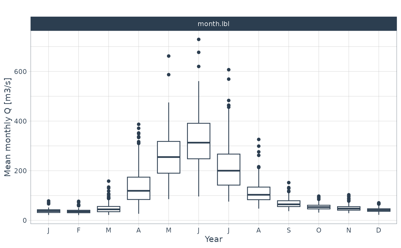
Monthly box plot of the time series data showing the mean (bold horizontal line), the boundaries of the 25% and the 75% quantiles (boundaries of the box). The lines extend to roughly 95% confidence interval and the points indicate outliers.

discharge %>% 
  summarise_by_time(.date_var = date, 
                    .by       = "month",
                    value     = mean(data)) %>% 
  tk_ts(frequency = 12) %>% 
  forecast::ggsubseriesplot(year.labels = FALSE) + 
              geom_smooth(method = "lm", color = "red", formula = y ~ x) +
              xlab('Month') +
              ylab('Mean monthly Q [m3/s]') + 
  theme_bw()

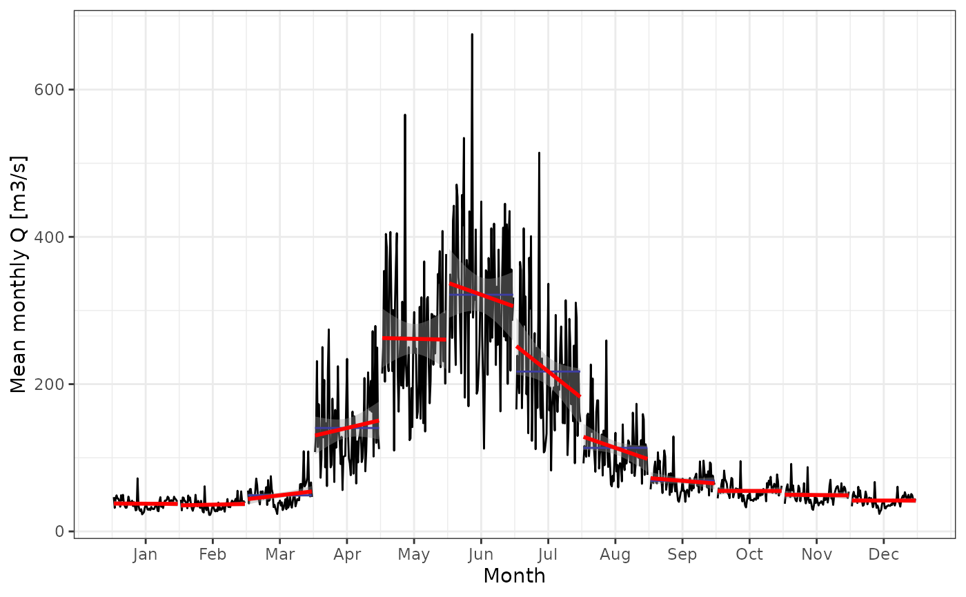
Visualization of trends in the monthly data. The blue line indicates the monthly mean and the red line shows the result of a linar model of the monthly data, including a grey confidence interval of the fit.

For many applications, discharge data is processed within the hydrolgoical year. In Central Asia, the hydrological year starts on October 1 of the previous year and ends on September 30 of the current year. Hydrologists also differentiate between cold and warm season discharge. The following function calculates mean annual discharges (ann) as well as mean cold and warm season discharge (cs and ws respectively).

# Convert the decadal data to monthly data
discharge_monthly <- aggregate_to_monthly(
  dataTable = discharge, 
  funcTypeLib = list(mean = "Q"))

discharge_processed <- convert2HYY(
  data2convert = discharge_monthly, 
  stationCode = 16279,  
  typeSel = "Q")

discharge_processed |> pivot_longer(-hyYear) |>
  plot_time_series(hyYear,value,name,
                   .title = '',
                   .x_lab = 'Year',
                   .y_lab = 'Mean monthly Q [m3/s]',
                   .interactive = TRUE,
                   .smooth = FALSE)

Mean annual (ann), cold (cs) and warm season (ws) discharge.

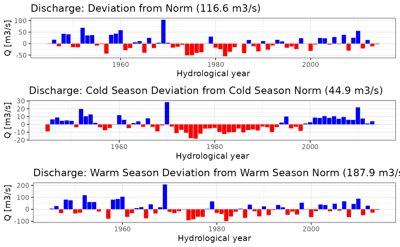
Also of interest may be the deviation from norm discharge over the years and seasons.

plotNormDevHYY(discharge_processed, "Q", "Discharge")